Nick's Auto-Evo Algorithm (Episode 1)

A small question: why do we need to calculate a species’ population within such small timesteps? Going through an editor cycle represents millions of years passing, and dividing all that up into something as small as months in order to figure out how an adaptation affects population seems a little inefficient.
I see how it could be interesting to see populations subtly change through the seasons as you play as a more long-lived organism. But I don’t think any organism gameplay will last much longer than a single generation, and for the most part species populations seem like they’d be mostly static throughout the gameplay phases of the game.

Good question, and it’s something that is explained fully in Episode 2, but here’s a quick overview.

The current population algorithm is not actually to use to calculate how the population will change over the many many months that there would be in millions of years of evolution. It’s only so that we have a way of measuring the “Performance” or “Fitness” of a species, since we’re defining fitness as that which gives the biggest boost to population growth.

The idea is we assign a mutation to a species, and then look at how that would affect its population growth over a simulation of X months (let’s say 120).

For example, say you have Species A. You create four sample groups of Species A, and assign a random mutation to each one (all these numbers are random):

  • Increase leg length by 10%
  • Increase digestive ability of stomach by 25%
  • Increase shoulder width by 20%
  • No mutation

Then for each of these sample groups, you run the Population Algorithm on them for 120 months to see how much it changes the population. The sample group that has the greatest growth is the winner.

The winner has its mutation chosen and applied to the species, and the game fast-forwards millions of years to the next generation of gameplay. If the winner was the group with no mutation, then the species does not evolve that generation.

It’s sort of like we have a car and we are designing a little test-track for it to drive on to simulate driving in the real world. Then we make changes to the car and see how it affects its performance on the test track to decide whether the change was good or bad for when it goes into the real world.

3 Likes

Part 2: Food

The ultimate and eternal goal of life might be reproduction, but the means to that is acquiring food. I can’t blame them, without it, you’re dead.

I know that the last part was very lengthy, so this one will be pretty brief. Recall the list of assumptions in the previous part. One thing I like to imagine as we work on this algorithm is the idea of cutting down that list of assumptions like peeling the layers of an onion. Every assumption we peel off takes us one step closer to the final, realistic algorithm, or the center of the onion. But we have to be careful and do it properly if we don’t want to break down into tears.

Remember in the demo from the last part that the population grew exponentially forever? In this part, we’ll start to address that by introducing the main limiter of life: Food.

From our current list of assumptions, here is the assumption we will address this part:
  • Modelus Specius is a flat, tiny, simple, jelly-like organism that lives at the bottom of the ocean.
  • The species is always fully satiated with food and water (Nutrition)
    • Which we will replace with:
    • Members of the species can instantly perceive food regardless of distance (Perception)
    • Members of the species can instantly teleport to perceived food (Movement)
    • Members of the species can completely consume the food and gain 100% of the energy. (Hunting/Metabolism)
  • The species is equally distributed/dispersed across the world (Demographics)
  • The planet is one giant ocean of equal pressure water that is equally accessible to the player (Geography/Terrain)
  • Members can reproduce as many times as they want, instantly, with no pregnancy/gestation period. (Reproduction)
  • The species reproduces via asexual reproduction, spawning fully developed offspring that can themselves immediately begin reproducing. (Mating)
  • The species does not change in physiology as they age (Aging/Ontogeny)
  • The species is fully aquatic (Terrestriality)
  • Members of the species are solitary and do not cooperate with other species members in any way. (Cooperation/Sociality)
  • The species has no parental instincts, and will immediately abandon offspring (Parenting)
  • The species is perfectly adapted to its environment and suffers no death or disease from environmental conditions (Environment)

Calories

The basic unit of measuring food and consumption will be the calorie (specifically the food calorie or kilocalorie). It can be used to measure the energy yielded from food and the energy needed by organisms to survive and do things. Every month, the species will have a total number of calories they need to eat. If they fall short of that number, then they lose some members to starvation. First let’s calculate the calories needed by the species.

Every species member will have a Base Metabolism, which refers to the standard amount of calories they will burn on a typical day just by existing. This is equivalent to a concept called Basal Metabolic Rate in biology, but is not exactly the same since our scenario is still so simplistic. Also, since our organisms are so simple, their base metabolism will not fluctuate day by day, since whereas in real life activities like hunting, hibernating, or reproducing can drastically change the amount of calories you burn.

Modelus Specius is a very small and simple organism, so we will give him a base metabolism of 10 calories per day, which comes out to 300 calories per month. Then we multiply this by the total population at a given timestep, and that gives us the total number of calories needed by the species at a timestep.

Calories Required = Base Metabolism * Population

Starvation

Since we are using averages, let’s say that the ratio of calories consumed to the calories required represents the proportion of the overall population that is fed (Proportion Fed). The species only eats as much as they require and no more, so Proportion Fed is capped at 1.00.

Say the species only consumes 75% of the calories they need. This makes the Proportion Fed 0.75. This could mean that 75% of the population receives all the calories they need and suffer no health consequences, and 25% receive no calories and die of starvation. However, this could also mean that 100% of the population only receives 75% of the calories they need, and as a result of the health consequences (aka diseases) they get from this, 25% of the population dies. So, in a way, these deaths are theoretically from starvation AND starvation-induced disease. The statistic could also represent any range of possibilities in between.

Let’s show how this would be represented mathematically:

Proportion Fed = Calories Consumed / Calories Required
Deaths from Starvation = Population * (1.00 – Proportion Fed)

Updating the Algorithm

Recall the current equations:

Deaths = Initial Population * 1 / Lifespan
Intermediary Population = Initial Population - Deaths
Births = Intermediary Population * Available Reproducers * Mating Frequency * Litter Size
Population = Intermediary Population + Births

Now we’ll add in deaths from starvation. Remember, the order of calculation is very important, so this is the order we will follow:

  • We start with the current population of the species
  • Next, all of the old species members die of old age
  • Next, all of the younger species members feed, and those who don’t die of starvation
  • Finally, all of the surviving species members reproduce

This is how that looks like:

Old Age Deaths = Initial Population * 1 / Lifespan
Intermediary Population 1 = Initial Population - Old Age Deaths

Proportion Fed = Calories Consumed / Calories Required
Deaths from Starvation = Population * (1.00 – Proportion Fed)
Intermediary Population 2 = Intermediary Population 1 - Starvation Deaths

Births = Intermediary Population 2 * Available Reproducers * Mating Frequency * Litter Size
Population = Intermediary Population + Births

And let’s visualize this with a Life Cycle Diagram:

Straightforward enough. There is one last thing we need to implement though, and that is where the calories come from. There are 3 different scenarios we can have.

Infinite Food

Food can be infinite, in which case we don’t track how much food is being consumed every timestep. We only care about the calories it provides the species. This essentially produces the exponential growth we saw in Part 1 since there is nothing to limit growth. This won’t be the approach we take.

Finite Non-Renewable Food

Food can be a limited/finite source. Eventually the calories will run out and the species will go extinct through starvation. This is also not the approach we will take, since it means the species will go extinct very quickly.

Finite Renewable Food

Finally, we can have food be a limited but renewing source. THIS is the approach we will go with, since it best simulates an ecosystem until we can start later adding in details like autotrophy and predation.

At this point, imagine the food to be individual little clouds of glucose floating in the water. We’ll say that each one yields 10 calories when consumed, and that the environment begins with 50,000 of them at the start of the simulation. Now let’s model this in the algorithm:

First, we calculate the total calories available from the food.

Calories Available = Food Amount * Calories per Food
Calories Required = Base Metabolism * Population
Calories Consumed = Calories Required OR Calories Available    #Whichever is smaller

Food Consumed = Calories Consumed / Calories per Food
Food = Initial Food - Food Consumed + Food Generated

Proportion Fed = Calories Consumed / Calories Required
...

And from this point on we’ve got the equations you saw above.

Calories Consumed will be capped by the total amount of calories available in the environment. Also, as the calories are consumed the amount of food is reduced. The food is also replenished at a steady rate every month (Food Generated).

Demo

With all of the equations finished, let’s plug into the demo and see the outcome.

Starting Conditions
  • Simulation Time = 24 months
  • Modelus Specius
    • Starting Population = 100
    • Available Reproducers = 1.0
    • Mating Frequency = 1/month
    • Litter Size = 1
    • Lifespan = 3 months
    • Base Metabolism = 300 calories/month
  • Food
    • Starting Amount = 50000
    • Calorie Yield = 10 calories
    • Regeneration Rate = 50000/month

There we go! Now the population is limited by the amount of food that is available in the environment. Notice that at first there is so much food available that Modelus Specius essentially grows exponentially. However, once the surplus runs out, famine hits and starvation rates cause the population to fall and stabilize at a much lower level. Interestingly, this is the furthest that most mathematical modelling of populations goes (except they sort of incorporate food with habitat space and other factors into an overall “carrying capacity” resource). So, from this point on, we are venturing into uncharted territories with the algorithm. It’s exciting to see how things develop!

This current model for food does assume many things to make it simple, and we will expand on these in the future to make the algorithm more realistic. These include:

  • Food is equally distributed between all species members with no competition
  • All the required food could be eaten on the last possible day of the month and still meet the monthly quota, instead of having to be eaten at regular intervals
  • No discrimination between food groups for calorie intake
  • There is no such thing as storing food either physically or through fat reserves

Summary

New Performance Statistics

Calories Required
Calories Consumed
Proportion Fed / Starvation Rate
Starvation Deaths

New Traits

Base Metabolism

Topics for Discussion

Suggestions and feedback are welcome!

3 Likes

May I suggest that we use KJ as the (primary) unit of energy, to better achieve the goal of being scientific. EU regulation 1169/2011 says that all food packaging needs to have the energy content said (first) in terms of kilo joules.

I’m liking this series so far. Recapping all the variables (showing the whole algorithm) is very nice. Hopefully at the end there’ll be some algorithm that can be quite easily converted into code.

Is this correct? Shouldn’t there be competition between species, as our model will act on a per species approach. Or are we going to get there in a future post?

2 Likes

Sure yeah we could make that change.

I’m making a Python script of the algorithm in parallel with posting the parts (I’m using it for posting the demos), so whenever anyone is interested I can send them a download link so they can see how it all works together.

By this I mean there is no intraspecific competition, i.e. that members of Modelus Specius don’t compete with each other for the food. They consume it on a first come, first served basis and leave leftovers for whoever’s after them. In one of the next few parts I’ll introduce how to replace this with more realistic models.


Also to anyone reading the thread, all feedback is welcome! Don’t feel daunted by not yet having read the full post. I’ve got the next part ready but I’ll wait a bit to give people a chance to give input on everything so far.

2 Likes

FOREWORD
Before I post the next part, I want to point out I had to spend a few hours debugging the auto-evo script because of the additions from this part. I finally figured out it was because of inconsistencies in the units. Some measurements were per month (like mating frequency), some were per second (like speed), and some were per individual while others were per the entire species. So I went through all the code and converted everything into SI units (the standard for science), and managed to finally fix it. It doesn’t really apply to you as the reader too much, but you might notice small inconsistencies with the numbers in Parts 1 and 2 with the future parts, and that’s because of this conversion. Anyways, on to the part!

Part 3: Movement

So far, the species has been hunting instantaneously, and therefore spending all of its actual time reproducing. Thus it was only limited in its growth by how often it could reproduce based on physical limits. Now let’s take the first step to fixing that and introduce some time dependence on hunting. This is the first step towards differentiating between the different life activities of the species and time spent between them.

From our current list of assumptions, here is the assumption we will address this part:
  • Modelus Specius is a flat, tiny, simple, jelly-like organism that lives at the bottom of the ocean.
  • Members of the species can instantly perceive food regardless of distance (Perception)
  • Members of the species can instantly teleport to perceived food (Movement)
    • Which we will remove and replace by actually tracking the time taken to reach food.
  • Members of the species can completely consume the food and gain 100% of the energy. (Hunting/Metabolism)
  • The species is equally distributed/dispersed across the world (Demographics)
  • The planet is one giant ocean of equal pressure water that is equally accessible to the player (Geography/Terrain)
  • Modelus Specius is the only species on the planet (Ecology)
  • Members can reproduce as many times as they want, instantly, with no pregnancy/gestation period. (Reproduction)
  • The species reproduces via asexual reproduction, spawning fully developed offspring that can themselves immediately begin reproducing. (Mating)
  • The species does not change in physiology as they age (Aging/Ontogeny)
  • The species is fully aquatic (Terrestriality)
  • Members of the species are solitary and do not cooperate with other species members in any way. (Cooperation/Sociality)
  • The species has no parental instincts, and will immediately abandon offspring (Parenting)
  • The species is perfectly adapted to its environment and suffers no death or disease from environmental conditions (Environment)

Instincts

We will now introduce the basics of instincts to the system. By this I mean we will make Modelus Specius prioritize certain activities at different times. For now, Modelus Specius will always prioritize hunting over reproducing (we will expand behaviours later). He will spend as much time as he needs to hunt, and then once he has gained all the energy he needed (or all the energy that was available), he will reproduce in the remaining free time.

This does introduce a dilemma. Is Modelus Specius’ reproduction passive or active? Can it occur in parallel with hunting? This currently assumes that the body waits until all the required energy is consumed, and THEN starts replicating its cells. Couldn’t the body start replicating cells earlier with the energy it had? We will address this in a future part when we discuss passive reproduction (releasing spores) versus active reproduction (searching for and courting mates). For now we will say that even though Modelus Specius reproduces through Budding which is typically a passive method, it is an active reproduction and cannot be performed while hunting.

Anyways, the introduction of movement doesn’t affect the life cycle diagram (so none of those this part), but it does allow us to create a new diagram, the Behaviour Diagram! It’s a breakdown of how the AI of Modelus Specius operates, i.e. how he spends his time. We can make a simple behaviour tree to visualize Modelus Specius’ instincts:

So in our model, hunting ALWAYS takes priority over reproducing until there’s either no more food, the time runs out, or all the required food is hunted.

Time per Hunt

Every hunt will take a certain amount of time. Every physics class talks about the standard formula of “speed equals distance over time”. Since we want to find the time spent for each hunt, we will instead write that as:

Time per Hunt = Distance per Hunt / Speed per Hunt

Let’s imagine the scenario. Let’s say that Modelus Specius is a small, spherical blob of simple tissue about 1cm in diameter. It uses a simple method of contracting its body to swim (undulation). Let’s say it swims at 10cm/s. It always knows where the food is. Once it comes into contact with food, it instantly consumes it and receives 100% of the energy. And finally let’s say that the patch is a perfect cube that is 10m long.

Edge Cases

This part can get a little tricky with the math and the logic, but I find that it helps to imagine things by thinking of the edge cases, such as when something is at 0% or 100% of its value. Keep this in mind as we continue.

Distance per Hunt

First we must find the average distance of each hunt. Imagine there was only one Modelus Specius and one piece of food in the patch (which is a cube), how could we know the average distance between them? This is actually a common puzzle in mathematics, and the solution is surprisingly difficult (involving a double integration). Luckily, it seems that the answer is that the mean distance between two points in a cube is 66% the length of the cube, and so of course this scales with the size of the cube. Please correct me if I’m wrong on this, because this is what I understood from reading the topic and is critical to the following calculations. This is how that looks mathematically:

Distance per Hunt = (0.66 * Patch Length) 

So in our 10x10x10 cube, the average distance between the Modelus Specius and the nearest (and only) piece of food is 6.6m.

NOTE
This is the first point of divergence for our algorithm between simulating microscopic and macroscopic species. Since the Microbe Stage is 2D, I’d imagine we would simulate the patches as squares not cubes, which makes the ratio 52%.

Okay, but when will a patch ever contain just one Modelus Specius and one piece of food? Now let’s imagine the opposite extreme scenario (here’s the edge cases trick I mentioned above). What if the entire volume of the patch is COMPLETELY filled, with half of the space being members of Modelus Specius and half being pieces Food, and they are evenly distributed between each other. What would the average distance be expected to be between each Modelus Specius and the nearest piece of food? Zero! Since they are literally packed shoulder to shoulder. So density REDUCES the average distance.

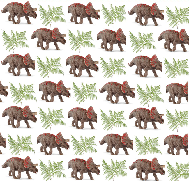
The Triceratops represents Modelus Specius and the Ferns the food. Imagine that they are physically filling up all the space in the patch. Notice that our model currently does NOT simulate population clustering. That is something we will address in a future part.

How do we mathematically represent density? We’ll show it as what ratio of the total volume of the patch is filled with the volume of Modelus Specius/the food. If 50% of the space in the patch is filled with food clouds, then that means the food has a population density of 50%.

So the average distance between Modelus Specius and the nearest piece of food ranges from it’s full value (at minimal density) to zero (at maximum density). Note that when I say maximum density I am referring to the densities of the predators AND the prey taking up all the space in the patch and being at a 50:50 ratio. If there is empty space in the patch, or if the ratio is imbalanced, than the average distance between predators and prey increases. This makes sense, since if the patch is 90% filled with predators and 10% filled with prey, some predators will be pretty far from the nearest prey (even if they are evenly distributed).

We can mathematically model this as:

Distance per Hunt = (0.66 * Patch Length) * (1 - (4 * Predator Population Density * Prey Population Density)) 

Why did I multiply the final term by 4? That’s so that when the predator and prey densities are both 50%, the average distance drops to zero. That will probably never happen in any playthrough though, due to many physical and other restraints. But it’s important so that the math works.

One last point to address. Our current equation measures the distance from the center of each Modelus Specius to the center of each food.

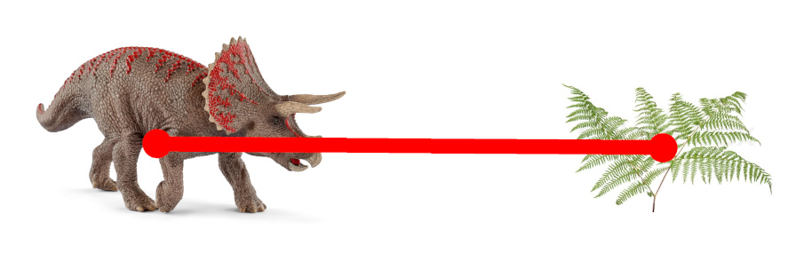
But Modelus specius consumes the food upon touching it, so we only care for the distance between the edges of their bodies, i.e. the red portion in the diagram below.

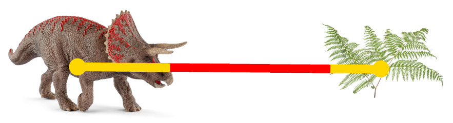
So, we must subtract the body radius of Modelus Specius and the “body” radius of the food from the distance, giving us the final equation of:

Distance per Hunt = (0.66 * Patch Length) * (1 - (4 * Predator Population Density * Prey Population Density)) - Predator Body Radius - Prey Body Radius

Speed per Hunt

Holy Belgium you wouldn’t think there’s so much work to just finding the average distance per hunt. Luckily the speed of the predator per hunt is very easy, since the food doesn’t try to escape. It’s just a constant we’ll apply for now that will be a trait of Modelus Specius (Swimming Speed), until we revisit swimming and hydrodynamics later. Let’s say his speed is 10cm/s, or 0.1m/s.

This gives us the following set of equations:

Distance per Hunt = (0.66 * Patch Length) * (1 - (4 * Predator Population Density * Prey Population Density)) - Predator Body Radius - Prey Body Radius
Time per Hunt = Distance per Hunt / Speed per Hunt

Time Spent Hunting

Now we must find the total time spent hunting every month. This value is PER INDIVIDUAL. Just because you have 2 lions doesn’t mean twice the time is spent hunting, because the lions will hunt simultaneously. So, we will calculate this next part by looking at the average individual member of Modelus Specius.

To find the total time spent hunting by the average individual, we just multiple the time per hunt by the number of hunts each individual needs to perform. Recall in the last part that we tracked the total amount of food consumed in the timestep. We are going to make a small tweak and change this into the food required, or in other words the hunts required. This represents the total number of hunts required by the population to feed themselves. This is important because now with movement speed, they may run out of time in the month to finish feeding!

If we divide the hunts required by the total population of predators we get the average number of prey/food that needs to be hunted by each predator, and since each hunt yields only 1 prey this also equals the number of hunts.

Hunts Required per Person = Hunts Required / Population
Required Hunting Time per Person = Hunts Required per Person * Time per Hunt

This gives us:

Distance per Hunt = (0.66 * Patch Length) * (1 - (4 * Predator Population Density * Prey Population Density)) - Predator Body Radius - Prey Body Radius
Time per Hunt = Distance per Hunt / Speed per Hunt
Hunts Required per Person = Hunts Required / Population
Required Hunting Time per Person = Hunts Required per Person * Time per Hunt

Successful Hunts

Remember that each timestep is 1 month. So we cap the maximum free time that an individual can spend hunting to 1 month. This means that if they require more than that, too bad, your time’s up. Think of it this way: If Jack needs to hunt 4 rabbits and he has 30 days to do it, but it takes 15 days to hunt each rabbit, sorry Jack you only get 2 rabbits.

Successful Hunts = Available Hunting Time per Person / Time per Hunt
Remaining Time = Free Time - Available Hunting Time per Person

This is a case that will be very unlikely to occur in our current simplified model though. It will become a more relevant concept as things get more complex.

Reproducing Time

Remember, we are tracking free time on the individual basis. So after the average individual finishes hunting, all the remaining time is used for reproduction. This gives us:

Reproducing Time per Person = Remaining Time

Which means we now tweak the births equation. Remember mating frequency gives the maximum births per month if you spend all month reproducing, but it has to be scaled down by how much time you can actually spend reproducing:

Births = Population * Available Reproducers * Mating Frequency * Reproducing Time per Person * Litter Size

Updating the Algorithm

At this point, the list of equations is growing long enough that I don’t think it’d be that helpful for me to just throw them all at you at the end of the part. If you really want it I can post it though. I’m also not really feeling the usefulness of the flow diagram. If someone wants it I can make it but otherwise I’ll ignore it for now.

Demo

However, the introduction of movement has now made the demo simulations a lot more interesting. Here is one using the conditions we discussed in this part. Note that some of these use different units in the calculations (the calculations use joules for example @hhyyrylainen ), but I’ve written them out here in easily understandable units.

Starting Conditions
  • Simulation Time = 24 months
  • Modelus Specius
    • Starting Population = 100
    • Available Reproducers = 1.0
    • Mating Frequency = 1/month
    • Litter Size = 1
    • Lifespan = 3 months
    • Base Metabolism = 300 calories/month
    • Swim Speed = 1cm/s
    • Body Radius = 0.5cm
    • Body Volume = 0.52cm^3
  • Food
    • Starting Amount = 50000
    • Energy Yield = 1 calories
    • Regeneration Rate = 50000/month
    • Body Radius = 5cm
    • Body Volume = 523.6cm^3

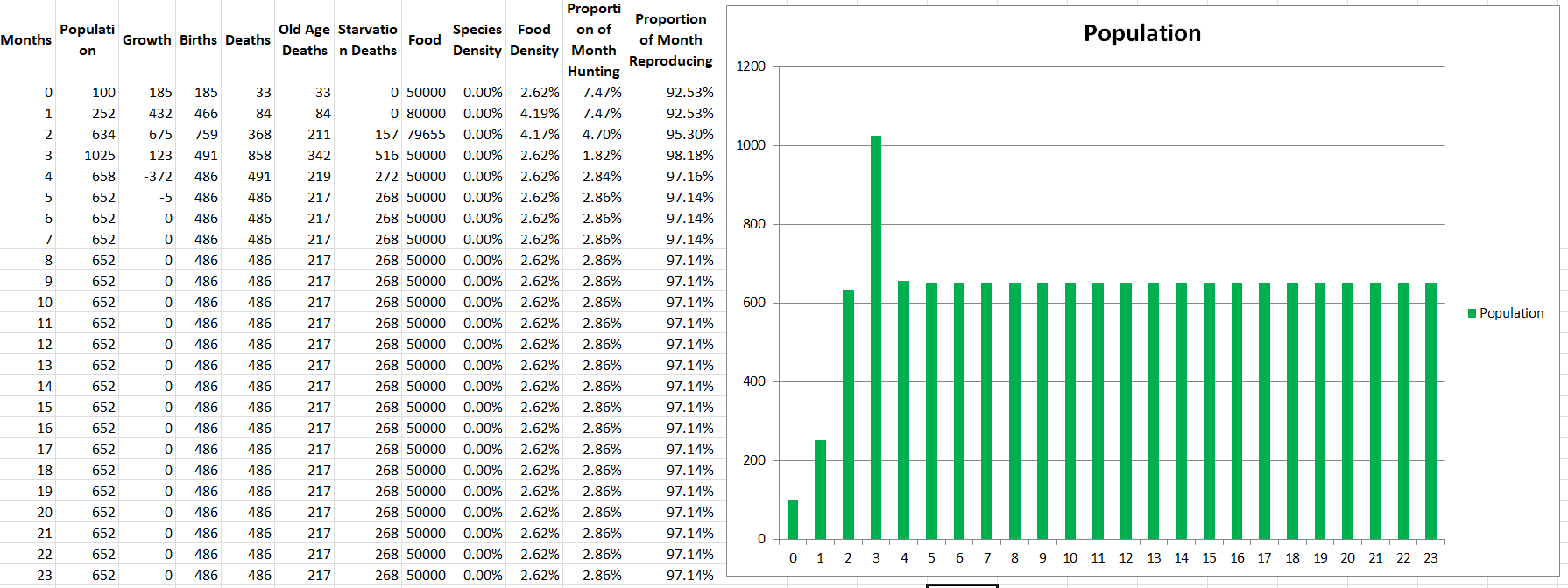
There are a few cool takeaways from the data. We can see that the population grows rapidly at first since food is in abundance, and then stabilizes at a lower level when shortages hit. We can also see that they are able to finish hunting so quickly that every month they still spend over 90% of their time reproducing. At first, they spend about 7% of their time hunting, but as their population increases the average distance to the food goes down and so they cut down to only spending 3% of their time hunting by the end. Also the species density is not actually 0%, it’s just a very small number that doesn’t show up. I will do a follow-up post to this one where I’ll explore different starting conditions and see what outcomes we get to better explore the simulation we’ve got going so far.


Summary

New Performance Stats
Population Density
Required Hunts
Successful Hunts
Distance per Hunt
Time per Hunt
Hunting Time per Person
Reproducing Time per Person

New Traits
Swimming Speed
Body Radius
Body Volume

Topics for Discussion

  • Can the mean distance between two points in a unit cube being 0.66 be scaled with the size of the cube?
  • How do we want to approximate a patch to be shaped as? A cube? A sphere?
  • In microbial gameplay, will we simulate patches as 2D?
  • Comments and feedback are welcome!
1 Like

Hi Nick, this is interesting to read. A few thoughts, sorry this came out really long unintentionally.

I really like the idea of breaking things down into Life Activities, that makes a lot of sense for working out how one change might impact a creature in different ways (like more armour improving combat but slowing grazing or something).

On the question of continuous Differential Equations and using tools from calculus vs Difference Equations (having discrete update steps as you are talking about) is that in terms of complexity they are much the same. Whenever you computer model a continuous Differential Equation you have to discretise first and then work with the corresponding Difference Equation. So the latter aren’t really any less complicated (though going with discrete time steps is the best way to go for us I agree),

In general with both these types of equations there is a tradeoff between complexity (and therefore accurately modelling the world if that is what you are trying to do) and analysis (being able to understand what the model will do) and control (being able to change the parameters of the model so that it gives you the behaviour you want). The more complex things become the harder it is to understand what is happening and the harder it is to control it.

Ultimately the thing we are giving the player is a control problem, which is: by changing your species blueprint (and other parameters like behaviour) can you get your population to a high level relative to the other species.

So if we use a highly complex model then the issue is that it will have chaotic dynamics and the player won’t be able to control it very easily. If you look at the Lotka-Volterra equations which are a very simple predator prey model you can see (just from looking at the graphs) that there are oscillations in the solutions. The model doesn’t converge to an equilibrium, it keeps changing over time.

This makes control quite a difficult problem. For example I could say “your pop is 25” which is the high point of a cycle and then you make some positive change to your creature and I say “your pop is now 13” which is the low point of a cycle, so you undo the change and I tell you “your pop is now 18” which then feels like it makes no sense and so you do no changes and I say “your pop is now 23”. It feels very random.

You can do things like averaging but once the dynamics become sufficiently chaotic that won’t help as there will be oscillations of many different frequencies.

In general your model has been mostly linear (which will converge to a stable equilibrium) however when you introduce this “Predator Population Density * Prey Population Density” you are introducing a non-linearity, which is going to start to lead you down the road to complicated, non-linear dynamics such as oscillations and chaos (which is in itself a really cool subject and a great thing to explore). Basically when prey is high predators will surge but then there will be too many predators so prey will collapse causing predators to collapse causing prey to surge etc.

So if you’d like to carry on with what you are doing feel free, I just kind of wanted to offer that as a warning that my guess about what will happen is as you introduce more non-linearities you will get more and more complex dynamics come out and it will become uncontrollable. However it might be a great learning experience to try it out for yourself and see what happens as you go further. I may also be completely wrong (that happens a lot) though differential equations was the subject of my PhD so I know something about them.

My most recent attempt at an auto-evo algorithm is here the basic idea is to have just an energy balance model. So for what you are doing it would be a bit like cutting everything out except just computing “at what level of population does food consumption = food generation or production” as that’s generally the equilibrium you are aiming for anyway.

The reason I think this might work well is it’s much more controllable, for example if you add another chloroplast then you get a little more light energy compared with the other species and that increases your population, if you take it off (and all other species stay the same) then the populations will all revert to what they were before you put it on, which makes it possible for the player to feel like they are controlling what is happening.

On top of this it will react to the patch conditions (which I think is the main goal), so patches with no sunlight will lose all their chloroplasts.

I am very open to further discussions and changes / switching to a new algorithm / merging ideas or anything really. Making the auto-evo system is really hard because firstly it’s a hard problem and secondly it’s very core to everyone’s expectations of how the game will work so there are a lot of different opinions from a lot of directions on whatever is produced (which is good I guess, it’s nice people care about the game :slight_smile: )

And yeah don’t let me put you off, I am enjoying reading what you are doing so if you continue to write it I’ll continue to read.

3 Likes

Everything about the balance of complexity, analysis, and control is very true, and something I thought about a lot going into starting this series. Ultimately I decided for it and these were the reasons I came up with:

  • I’m already starting to see some oscillations reminiscent of Lotka-Volterra interactions with different starting conditions for part 3. The oscillations always stabilize around a mean though. However if future additions causes them to no longer do so, as long as the oscillations are regular enough around a certain mean I’d suggest we take that mean as the final value for the population. If we make changes and it produces oscillations AND they are chaotic (or even getting increasingly chaotic every round) I think that’s a point we need to step in as designers and change the implementation of that part to ensure we build a system that can be understood.
  • In terms of analysis, I think it’s very important that the player understand enough but not all of what’s happening. By this I mean they should understand enough to be able to make smart decisions, but not enough that they can see through the entire apparatus and perfectly predict the best moves to make every time. It should be like chess, where there are many different options and the struggle IS to be able to think ahead and predict outcomes and plan responses.
  • Expanding on the above point, I agree that it can easily become difficult to analyze the impact of your changes to the algorithm, UNLESS you track many of the stats and values over time and display them to the player. Even now in just part 3, it can be hard to predict what or why things are happening if you just look at months and population, but with all the other data available it allows you to see for example that the food ran out, or that the species has to spend most of its time hunting and thus doesn’t have much time left to reproduce, or patterns like that. If we reach a point where there’s simply too much information to display to the player without overwhelming them, I think that’s another point where we as designers need to intervene and simplify the model.
  • In regards to the energy balance model you’ve made, I do like the approach and I think it greatly avoids the risk of chaos or lack of control, but from my understanding of it it lacks the depth or complexity I believe the auto-evo system should have. As the fundamental selling point of the first half of the game, I think the evolution system should be as detailed as we can make it within the bounds of balance and fun. Some recent games I have played have showed me that it definitely is possible to do this and still create a great game, such as Kerbal Space Program for rocket science, or Ymir for economics and city-building. I think the best part of creating a detailed system is that it creates a simulation, which can then produce realistic but new and unexpected outcomes which can surprise you on every playthrough (which I’m already starting to see a little bit of just at part 3), and produce more interesting interactions between its actors.
  • Worst case scenario, it’s much easier to take a system that is too complex and simplify it, than to take a simple model and make it deeper and more complex. In fact many of the upcoming parts are far less groundbreaking than what we’ve implemented so far. For example food turned this from an exponential growth model into something that stabilizes, and movement introduces the oscillating effect of different species densities as you pointed out. This early stage is similar to building the framework and foundation of the house. However many future parts will just be filling in the rooms of the house, and not increase the complexity too much. We’ve got a part coming up on hydrodynamics, which acts to ultimately limit the swimming speed of species, and then the part on perception ultimately just reduces the number of predator-prey interactions, since they won’t always know where the prey are.
  • Finally, even if we ultimately reject this approach and choose a different algorithm, I think it can teach us a lot about how to implement different features like swimming, population density, hunting, and more, and I do personally enjoy making the episodes and being able to play with the simulation.
3 Likes

I am very inspired by KSP too, that’s what I would like to push towards, a lego like set of building tools which the player uses to overcome complex and challenging scientific problems in a fun way.

I am not sure about this, I think the opposite might be true. However as with many things doing a bunch of experiments is a good way of proceeding.

Also on the issue of complexity I think it shouldn’t be so hard to find enough. Even simple games like the prisoners dilemma become complex and interesting when played iteratively between multiple agents with different strategies.

Awesome :slight_smile:

Yeah I think experimentation is our major benefit. Since we are building it iteratively and from such a simple original framework, we can keep track of the entire algorithm as we build it and intervene if it starts to get too chaotic or complex at any point.

Part 3.1: Simulation Demos

As I mentioned in the last part, we’ll now do a series of demos with different parameters to better explore the system we’ve created so far, and see how changes to traits affect the population of the species. Hopefully it can also give us a taste for what the finished Auto-Evo system will feel like in the game!

Before we begin, however, running these simulations was helpful since it helped me find to flaws with the algorithm’s design. Firstly, I realized that people should die of old age at the end of the timestep, not the beginning. If the lifespan for a species is 1 month or lower, the entire population will die of old age before they get to do anything, which doesn’t make any sense. This change doesn’t change anything other than fixing that problem, and I’m not really sure why I didn’t think of this earlier. Here is what the new Life Cycle Diagram looks like:

Which much more closely resembles the typical lifespan of an organism (birth, survival, reproduction, death from old age).

Secondly, I’ve renamed the Population Density performance stat to now be called Spatial Population Density, since it’s actually a measure of what ratio of space the population occupies. This is so that Population Density can refer to its actual meaning of a number of individuals per unit of area or unit of volume.

Finally, to make things more interesting, I’ve tweaked some of the stats of the Standard Simulation to make life more difficult for the species. Then the following changes will almost be an experiment to see which is the best mutation. In fact we’re basically playing as the Auto-Evo system here, since the system will assign random mutations to a species and see which one best increases its survival. First, let’s begin with our baseline, the Standard Simulation.

Simulation 0: Standard Simulation

Starting Conditions
  • Simulation Time = 24 months
  • Modelus Specius
    • Starting Population = 100
    • Available Reproducers = 1.0
    • Mating Frequency = 1/month
    • Litter Size = 1
    • Lifespan = 3 month
    • Base Metabolism = 300 calories/month
    • Swim Speed = 1cm/s
    • Body Radius = 0.5cm
    • Body Volume = 0.52cm^3
  • Food
    • Starting Amount = 50000
    • Energy Yield = 1 calories
    • Regeneration Rate = 50000/month
    • Body Radius = 5cm
    • Body Volume = 523.6cm^3

In the original scenario, the population stabilizes at 270 individuals. We’ve analyzed why it follows the pattern we see in the past part, but to recap: The population grows quickly at first due to an abundance of food, but then when shortage hits it stabilizes at a lower level where the rates of food consumption match the rate of food regeneration.

Simulation 1: Increased Mating Frequency

Starting Conditions
  • Simulation Time = 24 months
  • Modelus Specius
    • Starting Population = 100
    • Available Reproducers = 1.0
    • Mating Frequency = 4/month
    • Litter Size = 1
    • Lifespan = 3 month
    • Base Metabolism = 300 calories/month
    • Swim Speed = 1cm/s
    • Body Radius = 0.5cm
    • Body Volume = 0.52cm^3
  • Food
    • Starting Amount = 50000
    • Energy Yield = 1 calories
    • Regeneration Rate = 50000/month
    • Body Radius = 5cm
    • Body Volume = 523.6cm^3

The cells of Modelus Specius have evolved special proteins that greatly accelerate the replicating process, causing the cells to double their original number 4x as quickly as before to produce offspring organisms through budding.

In this scenario the population stabilizes at 767. It’s interesting to consider why an increase in mating frequency led to such an increase in population. It also seems like Modelus Specius spends less time of the month hunting. I think the main reason why we see the increase in population is that increased mating frequency means more births to offset the number of deaths from old age and starvation. In fact you can see that every year the majority of the population dies of starvation (600 of the 767), but the surviving 167 have so many offspring that it keeps the species alive. This is a very interesting strategy that I had never even considered so far, and keep in mind how simple our model currently is! It’s crazy to see how it can already start producing these interesting interactions.

Simulation 2: Increased Litter Size

Starting Conditions
  • Simulation Time = 24 months
  • Modelus Specius
    • Starting Population = 100
    • Available Reproducers = 1.0
    • Mating Frequency = 1/month
    • Litter Size = 4
    • Lifespan = 3 month
    • Base Metabolism = 300 calories/month
    • Swim Speed = 1cm/s
    • Body Radius = 0.5cm
    • Body Volume = 0.52cm^3
  • Food
    • Starting Amount = 50000
    • Energy Yield = 1 calories
    • Regeneration Rate = 50000/month
    • Body Radius = 5cm
    • Body Volume = 523.6cm^3

A mutation to the DNA for Modelus Specius’ budding has created the unique situation where it grows four buds simultaneously and then releases all of them, increasing the number of offspring produced per reproduction.

I ran the numbers on this and it produces the exact same outcome as the scenario above. At the moment litter size and mating frequency have effectively the same effect on the simulation.

Simulation 3: Lower Base Metabolism

Starting Conditions
  • Simulation Time = 24 months
  • Modelus Specius
    • Starting Population = 100
    • Available Reproducers = 1.0
    • Mating Frequency = 1/month
    • Litter Size = 1
    • Lifespan = 3 month
    • Base Metabolism = 150 calories/month
    • Swim Speed = 1cm/s
    • Body Radius = 0.5cm
    • Body Volume = 0.52cm^3
  • Food
    • Starting Amount = 50000
    • Energy Yield = 1 calories
    • Regeneration Rate = 50000/month
    • Body Radius = 5cm
    • Body Volume = 523.6cm^3

The cells of Modelus Specius have evolved a more efficient method of spending energy to perform processes in the body, and as such only require half as much energy (5 calories per individual per day) for their base metabolism.

In this scenario the population stabilizes at 548. Since the population consumes less energy at the start, it takes longer for the food shortage to hit so we see the population peak on the 5th month instead of the 2nd. My guess for the increase in population over the standard simulation is that since each individual only requires half as much energy, they only spend half as long hunting (2% of their time instead of 4%) which means they can spend that extra 2% of their time reproducing. It ALSO is because of the fact that with half the base metabolism as before, the environment now produces enough energy to support double the population.

Simulation 4: Increased Swim Speed

Starting Conditions
  • Simulation Time = 24 months
  • Modelus Specius
    • Starting Population = 100
    • Available Reproducers = 1.0
    • Mating Frequency = 1/month
    • Litter Size = 1
    • Lifespan = 3 month
    • Base Metabolism = 300 calories/month
    • Swim Speed = 10cm/s
    • Body Radius = 0.5cm
    • Body Volume = 0.52cm^3
  • Food
    • Starting Amount = 50000
    • Energy Yield = 1 calories
    • Regeneration Rate = 50000/month
    • Body Radius = 5cm
    • Body Volume = 523.6cm^3

Some cells on the edges of Modelus Specius have evolved some of their internal proteins into elastic fibres that can cause them to expand and contract at a greater range of motion. This allows the organism to undulate with wider motions and swim faster (from 1cm/s to 10cm/s).

In this scenario the population stabilizes at 277 (remember standard simulation was 270). I think this tiny increase is because so little time was being spent hunting anyways, that increasing speed by 10x barely affects the overall population. Yes in the last simulation the less time spent hunting increased population, but remember it also involved less energy being consumed overall which greatly increased the OVERALL population that could be supported. Here the population cannot grow any larger because starvation rates will keep it in check.

Simulation 5: Higher Food Energy Yield

Starting Conditions
  • Simulation Time = 24 months
  • Modelus Specius
    • Starting Population = 100
    • Available Reproducers = 1.0
    • Mating Frequency = 1/month
    • Litter Size = 1
    • Lifespan = 3 month
    • Base Metabolism = 300 calories/month
    • Swim Speed = 1cm/s
    • Body Radius = 0.5cm
    • Body Volume = 0.52cm^3
  • Food
    • Starting Amount = 50000
    • Energy Yield = 10 calories
    • Regeneration Rate = 50000/month
    • Body Radius = 5cm
    • Body Volume = 523.6cm^3

Chemical changes on the surface of the ocean have led to denser clouds of glucose floating in the oceans, containing 10x as much energy.

In this scenario, the population stabilizes at 2777. I know that this is technically not a mutation to the species but a change to the environment, but I wanted to try it too. We can see that increasing the energy yield of the food drastically affects the species’ population. It takes much longer for the food shortage to hit, so the population peaks on the 9th month instead of the 2nd. Also, each food cloud is so energy rich that each individual only needs to hunt 1 to receive all the energy they need for an entire month, drastically reducing the time they spend hunting. Since 50,000 units of food are produced every month, but the energy of that food has increased 10x, the environment can now support a much higher population with the energy it produces. For all these reasons (and maybe a few more I’m not thinking of), the population of Modelus Specius is effectively able to increase by 10x.

Final Results

Now we can look at the final population achieved with each mutation.

Obviously the Increased Food Energy Yield had the greatest effect, but let’s pretend we are Auto-Evo and that is not an option. We would choose Increased Mating Frequency or Increased Litter Size as the mutation for Modelus Specius, since it produced the greatest increase in population size.

Also keep in mind that the “strength” of those different mutations depended a lot on the conditions of the environment. Since energy was so abundant, lower base metabolism and increased swim speed were not as effective as adaptations, whereas increased mating frequency or increased litter size allowed the species to rapidly grow its population and make greater use of the plentitude of energy in the environment. Perhaps if energy was much harder to come by, lower base metabolism and increased swim speed would have been much better adaptations!

I hope you guys found that interesting and that it helped give a sense of how the algorithm works and how it will ultimately be used to guide Auto-Evo. It definitely did whet my appetite for seeing evolution in action in the final game. I think these demo simulations will only get more and more interesting as we add more elements to the algorithm. Next time we’ll be back with the next part in the series!

4 Likes

FOREWORD
After some thought and discussions on Discord, I’ve realized that this next part is actually mostly unnecessary. However, it’s worth discussing the parts of it that matter, so get ready for probably the shortest part of this series.

Part 4: Demography

As you can see, within just a few parts we’ve already quite rapidly created a rudimentary auto-evo algorithm, with traits like swimming speed, base metabolism, and mating frequency factoring into the survivability of species. I really like the approach we are taking because it feels like we are building the framework of the algorithm, and then filling in the details later. We will soon be ready to start introducing other species into the mix, but before we can do that there are two quick topics we must cover in their own parts.

The first is this part, on habitats and demography. How does where the species live affect its likelihood of interactions with other species? We have already factored in density, but there’s also other factors of the distribution of species in nature such as preferred habitats, habitat overlap, clustering, etc.

We will revisit other aspects of habitats again in the future, such as migrations, environmental conditions, territoriality, etc. For now though, we must simply consider where in the patch Modelus Specius is likely to live and how that affects its interactions with other actors in the patch.

We will be breaking down the following 2 assumptions from our list:
  • Modelus Specius is a flat, tiny, simple, jelly-like organism that lives at the bottom of the ocean.
  • Members of the species can instantly perceive food regardless of distance (Perception)
  • Members of the species can completely consume the food and gain 100% of the energy. (Hunting/Metabolism)
  • The species is equally distributed/dispersed across the world (Demographics)
  • The planet is one giant ocean of equal pressure water that is equally accessible to the player (Geography/Terrain)
  • Modelus Specius is the only species on the planet (Ecology)
  • Members can reproduce as many times as they want, instantly, with no pregnancy/gestation period. (Reproduction)
  • The species reproduces via asexual reproduction, spawning fully developed offspring that can themselves immediately begin reproducing. (Mating)
  • The species does not change in physiology as they age (Aging/Ontogeny)
  • The species is fully aquatic (Terrestriality)
  • Members of the species are solitary and do not cooperate with other species members in any way. (Cooperation/Sociality)
  • The species has no parental instincts, and will immediately abandon offspring (Parenting)
  • The species is perfectly adapted to its environment and suffers no death or disease from environmental conditions (Environment)

Questions to Consider

When addressing these two assumptions, there are a few questions that are raised:

  • What would a species’ habitat look like? Can it be assumed that a species occupies the whole patch? Or only parts of the patch?
  • If they only occupy parts of the patch, how do we calculate overlap?
  • Is the species evenly distributed across the entire habitat they occupy? Or are they clustered?
  • Are there inaccessible zones of the patch? (Physical barriers, isolated bodies of water, pressure differences, other physiochemical differences)

Habitats

What would a species’ habitat look like? Can it be assumed that a species occupies the whole patch? Or only parts of the patch?

From the definition of a patch, we are going to assume that all species in a patch occupy all parts of that patch. Habitats thus will not be defined by what parts inside of a patch are occupied by the species, but rather which specific patches are occupied in the first place. For example, consider the following diagram:

A species of camels would have their habitat defined by the 8 Desert patches that they occupy. However, within those patches the camels would be assumed to live in the entire area/space. This concept will be explored more in Episode 2.

Patches will tend to be smaller and represent a piece of land or ocean or sky that has very similar living conditions all across, so this is a fair assumption to make.

Overlap

If they only occupy parts of the patch, how do we calculate overlap?

This question is irrelevant because of the answer to the first question. Since we are not assigning specific habitats inside of a patch, overlap is unnecessary because all species in a patch will ALWAYS overlap. Therefore overlap will be more in regards to whether 2 species live in the same patch, and how many patches they live together in. This is something to revisit in Episode 2.

Clustering

Is the species evenly distributed across the entire habitat they occupy? Or are they clustered?

Here is an interesting point to consider. It might be difficult to imagine how clustering would affect demographics, so here’s a diagram to help illustrate the point.

image

Imagine a scenario with multiple species that fill up the entire patch, aka a case of high spatial density (remember that population density was renamed to spatial density). With even distribution, as seen on the left side, the average distance between any one species and the nearest member of another species is quite short, something we explored in part 3. When distribution is even, this is equivalent to minimal clustering (or a clustering value of 0).

When clustering is maximized (a clustering value of 1.0), all species are lumped into big groups. Notice how suddenly the average distance between any species member and a member from another species becomes much longer. For example the orange species members are now much further from the red species members.

So imagine you are a predator. Increased spatial density of your species and the prey species is a BENEFIT because it makes it more likely for a prey to be very nearby to you. Therefore, increased clustering diminishes the benefit of spatial density by grouping members of a species together, instead of allowing them to be mixed in. Another way of thinking about it: Increased density decreases the average distance to a prey, and increased clustering decreases the effect of density, therefore increased clustering increases the average distance to a prey.

On the flip side, when spatial density is low, clustering doesn’t really matter because there are fewer individuals (think of just 1 predator and 1 prey, clustering is irrelevant in such a case because there is no one to cluster with).

So this is the current equation for calculating the average distance between a predator and its prey, factoring in the spatial density of both species:

Distance per Hunt = (0.66 * Patch Length) * (1 - (4 * Predator Population Density * Prey Population Density)) - Predator Body Radius - Prey Body Radius

Now we’ll add in a term that diminishes the density term. First we calculating the Average Clustering between the two species, and then factor that into the overall equation:

Average Clustering = (Predator Clustering + Prey Clustering) / 2
Distance per Hunt = (0.66 * Patch Length) * (1 - (4 * Predator Population Density * Prey Population Density * (1 - Average Clustering))) - Predator Body Radius - Prey Body Radius

With the above equation, when density is high then high clustering can reduce its effect, but when density is low the level of clustering is irrelevant. Clustering can never actually make the average distance to a prey increase more than it normally would be, it can only reduce density’s effect of making it shorter.

NOTE: Clustering will be defined as a species trait. Why would a species ever evolve clustering? If you are a prey to many species, it will make it less likely for you to be found by predators since you can hide all your species members in a corner. Also, clustering will be necessary for cooperative social behaviours that we’ll introduce in a future part.

Inaccessible Zones

Are there inaccessible zones of the patch? (Physical barriers, isolated bodies of water, pressure differences, other physiochemical differences)

To this I would again say no due to the definition of a patch. A patch is defined as a contiguous space with common physicochemical features, so if there was a barrier that would define a separate patch. Thus we don’t need to consider this.

Filling up the Oceans

Finally, before we can close, there’s one more point to consider. The algorithm actually currently has no limit on the number of organisms that can exist in the patch. Modelus Specius could theoretically have millions of offspring and fill the oceans of the world multiple times over (if there was enough food). We should introduce a limitation in terms of physical space to prevent this from ever occurring.

We will do this by limiting births. If the number of births is ever going to produce more offspring than can physically fit in the patch, we will just limit it to what can physically fit. I’ll skip showing the math behind this because I think it makes sense already, but if someone wants to see the equations for it let me know.

Demos

There will be no demos this part, since the changes were so minor and barely visible in the results. I did notice though that increasing clustering did lead to either more time spent hunting, or lower overall populations for Modelus Specius because of less free time to reproduce.

As compensation for this less eventful part, the next part will be coming out pretty soon!


Summary

New Performance Stats
None

New Traits
Clustering

Topics for Discussion
All comments and feedback are welcome!

I realized I made a mistake with the corrected diagram at the top of this post. It should actually look like this:

In the updated algorithm, the first thing that happens is that the script determines what fraction of the population dies from starvation and kills them off first. Then of the remaining population, it determines how many offspring were birthed. Before it adds the births, it also kills off any of the population members who die from old age. Therefore births and old age deaths occur sort of in parallel.

Anyways, just wanted to make that clear and I’ll go back and fix the original post later. The next part will be coming up soon! Feel free to leave any suggestions or feedback you have on the series so far.

1 Like

Part 5: Hydrodynamics and Swimming

Yes we have a stat for movement speed now, but it’s a generic stat that is not tied to the organism’s body or the environment in any way. In this part we will look at the hydrodynamics of swimming and how to make movement speed realistically determined. There are no specific assumptions from our list that we are breaking down, instead we are just adding detail to the movement calculations from Part 3. Let’s find out how to make a creature’s swimming speed depend on its size, shape, and surroundings.

Undulation

Modelus Specius is a simple, spherical creature comprised of simple tissue. We’ll assume that this simple tissue has basic abilities to perform various tasks, such as in this case contracting to act like a muscle. We’ll classify Modelus Specius as using the type of swimming referred to as undulation, meaning it flexes the sides of its spherical body back and forth to propel itself forward. Thus we’ll say only the tissue on the sides of its body are contributing their force towards the swimming motion.

It’s hard to imagine how a solid sphere would use undulation, so imagine it as similar to the motion used by jellyfish (except that there is no hollow cavity or tentacles in the bottom).

Online, it says that the fastest recorded speed of a jellyfish is 8 kph. Dividing by ten I think gives us a more realistic top speed for small and simple jellies that are similar to Modelus Specius, so a top speed of 0.8 kph or 0.2 m/s. Now, for the next step, let’s take a look at Forces.

Force

Force is a simple concept in physics. It’s basically an interaction or energy that changes the motion of an object. When an object experiences a net force in a direction, it accelerates in that direction. When an object experiences no net forces in a direction, it maintains its motion in that direction (which could be maintaining its current speed without decelerating, or it could be being completely motionless). Keep in mind that accelerating in one direction (such as backwards) is the same as decelerating in the opposite direction (forwards). Why “net” force by the way? Because you can have multiple forces that act in opposing directions, but the ones that are greater will determine how the object’s motion changes.

For Modelus Specius’ swimming, we will consider its motion as an interplay of two forces: The “thrust” or “swim” force that the organism produces to propel itself forwards, and the drag force of water pushing back against it as it swims. We can visually display these using a diagram common in physics, a free-body diagram

image

Drag Force

At top speed, the swim force and the drag force will perfectly balance each other out, resulting in top speed being achieved and no more forward acceleration. Why is this the case? Because when you first start swimming, your Swim Force greatly outweighs your Drag Force. However, Drag Force increases with your speed, so as you speed up your Drag Force increased but your Swim Force stays the same. Eventually your Drag Forces reaches the value of your Swim Force, and that’s when you hit top speed and stop accelerating.

We already know the top speed of the Modelus Specius, which we’ve estimated at 0.2 m/s. But what if the ocean’s temperature changed and made water more resistant to swimming (higher drag)? What if Modelus Specius’ size got larger and less hydrodynamically shaped? Since drag force can vary so much, we should use our estimate of 0.2 m/s top speed to find the actual Swim Force produced by the jellyfish.

To find the Swim Force, we will find the Drag Force and know that by definition the Swim Force has to be the same value. Drag Force can be calculated using the following equation:

image
Let’s break this equation down variable by variable to see how drag will be calculated in Thrive.

Relative Flow Velocity

This refers to the difference of velocity (remember that velocity is just a physics term for speed with a direction) between the fluid and the object.

If the fluid flows in the opposite direction to the organism’s motion, then you add the velocities to find the relative velocity. If flowing in the same direction like the 2nd panel, you subtract them (if you and the water are both moving the same way, it feels like you’re not moving). If the water is motionless, you only consider the velocity of the organism. Okay, simple enough, but this brings us to a dilemma.


The Dilemma

Now obviously ocean currents are a very real phenomenon that play a big role in life, but I simply cannot imagine how to make an algorithm that takes into account the role of water currents, especially when most of the values being used are averages. Water currents flow in different directions at different speeds all over the ocean. Do we just take an average direction and average speed for the entire patch’s water current?

Okay, say we do that, how do we factor that into the algorithm? Do we apply that to the speed of the organism when he is hunting? How do we know when the water current is flowing in the same direction as the movement? In the opposite direction? How do we know when it’s flowing at a 30 degree angle from the organism’s motion. We could theoretically get an “average direction” for all hunts, but how would that be calculated? We’d have to get an average position for the predator population, and an average position for the prey population. And keeping track of the positions of objects in the patch opens a WHOLE new can of worms…


There are two possible solutions I see to this problem:

  1. Completely ignore ocean currents and always assume the fluid’s velocity is 0.
  2. Completely ignore ocean currents within a patch, but consider ocean currents between patches.

Ignoring Ocean Currents

This is a simple solution that makes it so that we always only consider the velocity of the organism.

Ocean Currents Between Patches

In this scenario, you do the same as in the first solution, but instead you track ocean currents between patches. This means that ocean currents can affect things like migrations between patches, or even moving to another patch to hunt (if that is intended to be possible), but not any interactions within a patch. I feel like this solution doesn’t sacrifice too much realism since ocean currents play a more important role on the larger scale (between patches) than the smaller scale (within patches).

For our purposes, we will proceed using the 2nd solution, which means the relative fluid velocity is equal to the velocity of the organism, which is 0.2 m/s. This gives us so far:

Drag Force = 0.2^2

Density of the Fluid

Next we must consider the density of the ocean. The density of ocean water on the surface is 1027 kg/m^3. As you go deeper, the density of seawater increases. However, it increases at different rates depending on what latitude you are at. Seawater at latitudes of around 30-40 degrees south (a region called the Pycnocline) follow this pattern:

Modelus Specius lives at the bottom of the ocean, so let’s say the depth of the patch is 4000m. Assuming similar conditions to Earth at 30-40 degrees south, this gives us a density of 1028 kg/m^3. This means drag force is now:

Drag Force = 1028 * 0.2^2

We can simplify this and divide it by 2 (to get rid of the fraction in the formula) to get:

Drag Force = 20.56

Reference Area

When you swim into a certain direction, even though you are a 3D shape you are presenting a 2D profile or “silhouette” to the water. This “side” or “face” depends on which side you swim with, aka where is your front. Since Modelus Specius is a sphere, the frontal surface area is just a circle. In fact for a sphere any direction you look at it its 2D profile is just an equally shaped circle. Using the radius of Modelus Specius which we earlier defined as 0.5 cm, that gives us a circle area of 0.000079‬ m^2. This gives us:

Drag Force = 20.56 * 0.000079<U+202C> = 0.0016

Drag Coefficient

The drag coefficient is a value that takes into account the shape and texture of the object for how much drag it experiences. Many tests have already been done to find the Drag Coefficients for many reference shapes:

The Organism Editor will look at any species and assign the nearest approximation of drag coefficient based on what shape the front-side is closest to. Evolutions to skin (like hydrodynamically shaped scales) can increase or reduce the drag coefficient. Since Modelus Specius is a solid sphere, we’ll use the drag coefficient of 0.47.

Drag Force = 0.0016 * 0.47 = 0.00076

And that’s it! Our Drag Force is 0.00076 Newtons (the unit for force, also shortened to N). This means Modelus Specius must generate 0.00076 N of Swim Force.

Swim Force

When a muscle flexes, it produces a certain amount of force based off of the cross-sectional area of the muscle. Therefore if you know the area of the muscle, and since we know the force produced per area, you know the force the whole area can produce. Well for Modelus Specius it’s backwards, since we know the total force it can produce, and the total area involved in undulation, we can work backwards to find the force produced per area.

An example of cross-sectional area of human muscles.

A total of 0.00076N of force is being produced to swim when at top speed. The cross-sectional area of Modelus Specius is 0.000079‬ m^2. However, for realism’s purposes I would say that perhaps only 50% of the cells in the sphere are flexing and unflexing to produce the swimming motion, so that means half of that area so 0.000039 m^2. This gives a force per area of 19.5 N/m^2. Human muscle has a force per area of 350000 N/m^2. Yes, a lot more, but humans have also had millions of years to evolve their muscles to become incredibly efficient, whereas Modelus Specius is a very primitive species with very simple muscle fiber cells.

Updating the Algorithm

So now we have some values that we can put into the algorithm. Muscle Area (the area of cells involved in undulation), and Muscle Strength (the Newtons produced per area of the muscle). An organism uses these to produce Swim Force. Swim Force is then compared to the Drag Force caused by the environment, and the result determines the top speed of the organism.

One assumption this is making is that the organism will accelerate so quickly to its top speed that we can just use the top speed for its hunting speed, and ignore the time spent accelerating. For now we will have to make this assumption for simplicity’s sake, but in the future we can revisit this to try to flesh it out.

Demo

Running the updated algorithm gives us results very similar to Parts 4 and 3:

Starting Conditions
  • Simulation Time = 24 months
  • Modelus Specius
    • Starting Population = 100
    • Available Reproducers = 1.0
    • Mating Frequency = 1/month
    • Litter Size = 1
    • Lifespan = 3 months
    • Base Metabolism = 300 calories/month
    • Clustering = 0
    • Locomotion = Undulation
      • Muscle Area = 0.000039 m^2
      • Muscle Strength = 19.5 N/m^2
      • Drag Coefficient = 0.47
      • Frontal Surface Area = 0.000079 m^2
      • Swim Speed = 20cm/s (Derived from above above traits)
    • Body Radius = 0.5cm
    • Body Volume = 0.52cm^3
  • Food
    Starting Amount = 50000
    Energy Yield = 1 calories
    Regeneration Rate = 50000/month
    Body Radius = 5cm
    Body Volume = 523.6cm^3

The population stabilizes around 277. The reason not much changed is that many of the changes we’ve made were under the hood, supporting more advanced interactions with other species and the environment in future parts. For example, we can now make environmental changes to the density of the oceans, or evolutionary changes to Modelus Specius’ body, and it will change the speed of its swimming. Something that did change though is that the speed of Modelus Specius is now around 20cm/s instead of 1cm/s, which has reduced the time they spend hunting every month to even less (0.22%).

Glad to be done with this pretty technical and not very rewarding part. Next time, we will finally, finally add in the main ingredient of evolution that we all love… Other species!


Summary

New Performance Stats
None

New Traits
Locomotion Type
Muscle Area (Swimming)
Muscle Strength (Swimming)
Coefficient of Drag
Frontal Surface Area

Topics for Discussion

  • How do we model ocean currents?
4 Likes

FOREWORD:

The addition of new species warranted some big changes to the algorithm’s code. Not only does Auto-Evo now have to loop through several species to run calculations every month, it also introduces new “race” mechanics to see who gets food first. These new features were much more complicated than I originally anticipated, and I basically learned the hard way why it’s so important to organize your code. I had to do an overhaul of the code to make it cleaner and more organized to add in the new features. I also had to greatly increase how much data was being displayed in the final reports to make them show a lot more information and use them for bugfixing. This way we can see much more detail into what is happening month by month and use it to debug the algorithm whenever I make a mistake (which I made a lot of when implementing these new features). There may have to be a part or two after this for bugfixing of the script if I catch any more. Anyways, all the major bugs have hopefully been ironed out, so time to showcase the next part!

Part 6: Competition

So far in the series, we’ve created a single species that eats, swims, reproduces, and inhabits certain parts of the patch based off density and clustering. But that’s not how evolution works, with just a single species. Evolution pits multiple species against each other! I think it’s time to start adding in some competition!

In this part we will be removing the following assumption from our list of assumptions:
  • Modelus Specius is a flat, tiny, simple, jelly-like organism that lives at the bottom of the ocean.
  • Members of the species can instantly perceive food regardless of distance (Perception)
  • Members of the species can completely consume the food and gain 100% of the energy. (Hunting/Metabolism)
  • Modelus Specius is the only species on the planet (Ecology)
  • Members can reproduce as many times as they want, instantly, with no pregnancy/gestation period. (Reproduction)
  • The species reproduces via asexual reproduction, spawning fully developed offspring that can themselves immediately begin reproducing. (Mating)
  • The species does not change in physiology as they age (Aging/Ontogeny)
  • The species is fully aquatic (Terrestriality)
  • Members of the species are solitary and do not cooperate with other species members in any way. (Cooperation/Sociality)
  • The species has no parental instincts, and will immediately abandon offspring (Parenting)
  • The species is perfectly adapted to its environment and suffers no death or disease from environmental conditions (Environment)

We will start by adding one additional species to the environment. This species will have the exact same stats as Modelus Specius and feed on the same floating clouds of glucose. At the moment this is effectively equivalent to doubling the starting population of Modelus Specius, since they are both evenly matched. However instead of reaching an equilibrium with all of the population being in Modelus Specius, it will evenly split between the two species. After updating the algorithm, we’ll differ the stats of Species B to see if the environment reaches an equilibrium between the two species.

Then, once we have ironed out all the features of having two unique species in the environment, we will add two more species, and they will be given unique stats as well. Our goal is to create a simple environment of different species, that will serve as the foundation for the work we do in the future parts.

Also before we start, I tweaked some of the numbers of Modelus Specius to produce some more realistic outcomes for some of the statistics. Now the fraction spent hunting every month usually comes out closer to 30% of the month rather than 0.7%.

Summary of the changes
  • Mating frequency was reduced by 50%
  • Lifespan was increased to 12 months
  • Base Metabolism was increased to 100 calories a day
  • Muscle Strength reduced to 2.5N/m^2 (making the typical speed 7cm/s)

New Definitions

One more thing before we start the algorithm, it’s important to clarify the meaning of some terms I’ve been throwing around lately. I’ll add all of these entries to the glossary:

  1. Generation: A generation refers to a “turn” in the game. For example, when you start the game you are playing on the first generation of your species. After reproducing, entering the editor, and a timestep passing, you resume play in the 2nd generation. Technically, yes, you could say that there’s thousands of generations that would’ve occurred in the thousands of years that passed during the timestep, but for the game’s purposes we call the time after each editor session a new “generation”.
  2. Timestep: The time between generations is called the timestep. When a player enters the editor, does his stuff, and then returns to the game, the game fast forwards thousands or millions of years to represent the evolution that took place. That’s called a timestep. Every time the player reproduces and enters the editor, another timestep passes. Timestep just refers to the time that passed.
  3. Simulation Step: This simply refers to the unit of time for simulation for the population algorithm. At the moment, this is one month. This means that all the calculations are run over the course of a month, and then repeated for however many months that we want the simulation to go for.

If there are any questions or suggestions about these definitions let me know. Anyways, on to the calculations!

Order of Calculations

One point I’ve been bringing up a lot is that the order of calculations is very important… Well it’s time to bring it up again! We are now going to have several species running inside the simulation at once, so the order of calculation is critical for decisions such as who gets first access to food.

Turn Order

My original idea was to use a “Turn Order” to handle the multiple species. This is because of the way the algorithm is designed, where we calculate the population change of one species at a time over one month, and then repeat that however many months. At the end of a generation, the game would randomly pick a turn order for all the available species, and then every month it would run once through that list in the order they were assigned, running the population algorithm on each species. This meant that if a species was lucky enough to be at the top of the list, he’d feed first every month of a simulation before anyone else. This also meant that in times of shortage the bottom species on the list could get no food and immediately go extinct. I originally thought this was fair since it was random every time, so everyone had a chance of going extinct and on a future generation a different order of species could be picked, where perhaps you’re at the top. However, I realized that this was not allowing for the species to actually compete with each other in times of shortages.

Simultaneous Simulation

So instead, I decided to implement a simultaneous “race” whenever there is a shortage of food. In any month that there is more food than food that is hunted, the race mechanic is irrelevant and everyone gets the food they want. However, whenever there’s a shortage, the Success Rate of each species hunting the food determines what fraction of the food they get. For example, if Modelus Specius and the other specius combined want to hunt 10,000 food, but there’s only 1,000 food remaining, then if Modelus Specius has a success rate of 75% he gets 75% of the 1,000 and the other species gets the remaining 25%.

How do you calculate Success Rate you ask? Let me explain.

Race for the Food

Let’s first define the two species we have. We have Modelus Specius, the species one we know and love, and now we’ll introduce a second species called Propagatus Maxima. For now they will have the exact same stats. We’ll define a new statistic called Competitiveness, which will be used to calculate the success rate of each species in hunting the food.

Speed

We have no combat in our simulation at the moment, so competing for food is purely determined by who’s the fastest to get it first. We’ll represent this by having the species’ speed compared to the combined speed of all the other species. If Modelus and Propagatus have the exact same speed, say 1m/s, then each wins 50% of the contests. Here’s the mathematical form:

Success Rate = Speed of Modelus / ( Speed of Modelus + Speed of Propagatus)
Success Rate = 1 / (1+1) = 1 / 2 = 0.5 = 50%

However, if Modelus had twice the speed of Propagatus, he would win a larger share of the contests (in this case 2/3).

Success Rate = Speed of Modelus / ( Speed of Modelus + Speed of Propagatus)
Success Rate = 2 / (2+1) = 2 / 3 = 0.67 = 67%

So the greater your speed compared to the competition, the larger share of contests/races you win. Interestingly, with this equation no matter how fast your competitors are you’ll always get at least some of the food (representing hunts where you get lucky).

Population

Okay, but what if the slower species outnumbers the faster one 10:1? Shouldn’t that give a competitive advantage to the larger population since there’s more of them? Yes, so let’s introduce that into the mix.

Say cheetahs and hyenas both hunt antelopes. The cheetah can easily catch an antelope before a hyena 90% of the time because of his speed advantage. But, there’s only 1 cheetah whereas there are 100 hyenas. After that cheetah catches his first antelope, he doesn’t compete with the hyenas anymore and they’re free to now chase antelopes completely uncontested.

We’ll model this by having the Required Hunts of the species multiplied by its speed in the equation. If a species requires a lot of hunts, they’ll be competing for the prey a lot more and thus increasing their competitiveness. A species that is faster but requires less hunts will be like the cheetah and leave the competition early once they get their fill.

This does make a big assumption, and that is that there is no intraspecific competition (competition between members of the same species). I have avoided that so far since I cannot think of a good way to implement it, so please pitch in if you have any ideas on how to model it mathematically.

Say Modelus has twice the speed but Propagatus requires twice the hunts, this will look like:

Success Rate = (Speed of Modelus * Required Hunts for Modelus) / (Speed of Modelus * Required Hunts for Modelus + Speed of Propagatus * Required Hunts for Propagatus)
Success Rate = 2*100 / (2*100 + 1*200) = 200 / (200+200) = 200/400 = 0.50 = 50%

Their two advantages balance out and they both win half the contests. If one species had double the speed and double the required hunts, they’d win 80% of the contests (4x the success rate of their competitor).

Priority

One final component we are missing though. Two species could both have the same speed and same required hunts, but different Priorities for their prey. The cheetahs do all their hunting on antelopes, while the hyenas spend half their time hunting antelopes and the other half hunting zebras. Priority is a proportion simply representing what fraction of their energy they try to get from a given prey. This gives us the final form of the equation:

Success Rate = (Speed of Modelus * Required Hunts for Modelus * Modelus Priority for Food) / (Speed of Modelus * Required Hunts for Modelus * Modelus Priority for Food + Speed of Propagatus * Required Hunts for Propagatus * Propagatus Priority for Food)

Note that at the moment, there are only two species and they both chase after the same food, so they both have a priority of 1.00 for the food. In the future, we’ll create more complex food webs with predators having multiple different preys, so Modelus Specius could have for example a priority of 0.5 for Prey 1, 0.3 for Prey 2, and 0.2 for Prey 3 (all of a predator’s priorities must add up to 1.00).

To recap, we calculate the Competitiveness of a species for a given prey, and compare that to the Pooled Competitiveness of all predators hunting that prey. Using this equation, we can determine the success rate of two or more predators that hunt for the same prey based off their speed, required hunts, and prey priorities. In times of shortage, the success rate determines what fraction of the food they receive.

Competition is a Lose-Lose

If you have studied some biology you might know, competition is a lose-lose for both parties involved. Not only does competition harm you during times of shortage, but it also interferes in times of plenty as well.

We will get to the other interactions listed on that chart in future parts. For now we’ll discuss competition.

Assume that you are Modelus, and there is an equal population of Propagatus in your patch that is perfectly even in all stats. You both hunt for the same clouds of glucose. Statistically speaking, half the time you are likely to have a member of Propagatus beat you to the food you are chasing, and have to start a new chase. So even when food is in abundance the competition increases the time you need to spend on every hunt. We will also model this using Success Rate. If the two species are perfectly evenly matched in speed, required hunts, and prey priority, you will only have a Success Rate of 50%. If you are only winning 50% of the hunting contests, your average hunting time increases by 50%. This is because you need to hunt twice as much, since half your hunts are failing, to get the amount of food you need. If you are winning 90% of the hunts, then your average hunting time only increases by 10%. Recall the equation for Time per Hunt:

Time per Hunt = Distance per Hunt / Species Swim Speed

We’ll now update this to:

Time per Hunt = (Distance per Hunt / Species Swim Speed) * (1 / Hunting Success Rate)

NOTE: Hunting Success Rate is an average of the hunting success rates for all the preys that a species hunts. It is weighted by how many hunts are performed on that prey.

So we can see that even with ZERO shortage, competition increases the time spent hunting for all predators, even if any of the predators have an advantage. This should lead to a phenomenon observed in biology called the Competitive Exclusion Principle, which says that competition between multiple species for a single role will ALWAYS lead to one species winning and the others going extinct or evolving for different roles/niches. We will discuss this more when we run the demos.

The diagram above gives a simple illustration of the Principle.

And that’s all for the mathematical explanations of this part. Even though these explanations were shorter than previous parts, I probably spent 10x longer actually coding the prototype for this part, because of the complexity of the newly introduced interactions.

Demo with 2 Equal Species

Without further ado, let’s see how the introduction of new species changes the simulation! We currently have two species, Modelus Specius and Propagatus Maxima, and they have the exact same stats in all respects. Let’s see the starting conditions:

Simulation Conditions

image

Patch

image

Food

Modelus Specius

Propagatus Maxima

Running a demo of the two species produces the exact outcome we would expect, they perfectly match each other in population size the entire simulation, stabilizing at 446 members each. It’s not even necessary to show the graph for this demo, but at least we know the code is working as intended so far.

Demo with 2 Unique Species

Now for the one we were waiting for, where we assign different stats to each species. We’ll start by doing a very, very small change. We’ll simply increase the strength of Modelus Specius’ muscles from 2.5 N/m^2 to 3.5 N/m^2. A harmless evolution, right?

Propagatus Maxima went extinct in 21 months, while Modelus Specius survived and thrived and stabilized at 923 members.

So what’s the story. We can see the exponential growth at the beginning as there is an abundance of food. Notice that Modelus always seems to grow a little faster than Propagatus. Then the food shortage kicks in on the 8th month, and both populations lose a lot of members. However, Propagatus never recovers! Why is this? It’s because when there is an abundance of food competition increases the time spent to hunt but everyone gets all the food they need eventually (unless it takes them sooo long that they run out of time in the month). However, after the shortage starts, there is only so much food to go around every month. Modelus’ slight speed advantage lets them win more of the scarce food on month 9, which leads to a bigger gap between the two species’ populations by month 10. This bigger gap allows Modelus to win even more of the food, and the cycle continues until Propagatus goes extinct. What does this remind you of? That’s right, the Competitive Exclusion Principle. This is a perfect example of the principle in action, since both species are hunting the same “Food” which makes them competitors for the same niche.

A niche is akin to a “role” of a species in an ecosystem, defined by where it lives, what it hunts, and other such factors.

Interesting to note that even such a small competitive advantage of Modelus Specius over Propagatus Maxima builds up to a huge difference in population, and will eventually lead to Propagatus going extinct. This is exactly what is described by the Competitive Exclusion Principle, and it’s fascinating that this pattern emerged without us even specifically trying to put it into the algorithm. We simply modelled realistic interactions and have started to produce a realistic system! I have high hopes for where this algorithm can go!

Just a quick aside, now that we’ve got multiple species I’ll probably skip showing the tables with the monthly statistics since it would just be way too much information (since it’s one table for every species). I can keep posting them though if you guys really want them. For now though, I’ll show you Modelus’ report just so that we can understand what is happening:

What are some of the interesting patterns you see? Well for one thing you can see that the time per hunt goes down every month, and this is because Modelus is facing less and less competition as Propagatus dies off. This gradually leads to them having more free time to reproduce, which increases their birth rate and helps them reach a higher population.

One thing this demo has taught me though is that I feel that the starvation penalties may be a bit too harsh.

Less Severe Starvation Rules

At the moment, 100% of the starving population of a species will die next month. This leads to very sudden extinctions when food runs out. I know that making this value any less than 100% seems very unrealistic since it seems like you’re saying species members can survive over a month without eating. To counter that, I’d say that this percentage can also represent how much energy ALL species members are receiving. 75% Proportion Fed could also mean that ALL species members only receive 75% of the energy they need. So to create a bit of a “softer landing” for species that run low on food, and not letting them go extinct extremely quickly, let’s try making it so that only 50% of starving species members will die. This means starvation is of course still bad but not the game-ending event it was before. This means that your species could technically eat 0 food for an entire month, and only 50% of them would die. Is that entirely realistic? I’m not sure, but we cannot make any more granular changes unless we make the timesteps smaller, and perhaps this is better for balance. Let’s see how this affects the simulation with the same conditions as before.

There we go, a much less severe drop for Propagatus. Even though he looks like he is still destined to go extinct under the current conditions, he at least won’t do so in under 2 years. We can play with the severity of starvation to get the results we like, so I’ll leave that open as a discussion question.

How severe should starvation be?

One more demo with 2 species. This time let’s make Propagatus Maxima into the species he was intended to be. Modelus Specius’ strength will be set back down to 2.5, but instead Propagatus will have 20% higher mating frequency than Modelus.

Holy cow. Clearly increasing mating frequency appears to still be very overpowered. We can revisit potentially balancing that in a future part.

This has been a lengthy post, but luckily with lots of cool new content! We are finally starting to see a lot more of the typical patterns we associate with evolution emerge in the system. I will do a sub-part soon where I’ll crank up the number of species in the simulation to 4, giving each of them unique advantages, and we’ll see who wins the game of evolution! Then after that, we’ll proceed with the next part of the series. Until then, please leave your feedback below!


Summary

New Performance Stats
Competitiveness
Pooled Competitiveness

New Traits
None

Topics for Discussion

  • How do I model intra-specific competition (competition within a species)?
  • Is it possible to make the time-steps smaller? This would allow for more realistic hunger/starvation modelling. Except this could also make the algorithm very computationally intensive.
  • How severe should the consequences of starvation be? 100% death rate of all starving members?
2 Likes

I think there’s a typo here.

Very interesting to see multiple species added. I’m currently working on the basic framework for auto-evo (scheduling background calculations, waiting for them to end). It’ll soon be time to add some kind of fitness calculation.

1 Like

Interesting stuff.

So say you had only one limited food source in a patch, like iron maybe. Are you saying (assuming no predation) that even if you started with 100 species all but one would go extinct? And even if that one splits one half will just die off? I’m not sure that’s particularly ideal.

On the wikipedia page you linked to it says:

Competitive exclusion is predicted by mathematical and theoretical models such as the Lotka-Volterra models of competition. However, for poorly understood reasons, competitive exclusion is rarely observed in natural ecosystems, and many biological communities appear to violate Gause’s law. The best-known example is the so-called “paradox of the plankton”.[7] All plankton species live on a very limited number of resources, primarily solar energy and minerals dissolved in the water. According to the competitive exclusion principle, only a small number of plankton species should be able to coexist on these resources. Nevertheless, large numbers of plankton species coexist within small regions of open sea.

I imagine that we would want a bunch of different plankton-like species right all coexisting?

1 Like

Ah thanks I fixed the post.

Also very interesting, what are you planning to include in the fitness calculations? Let me know if I can offer any of the equations or functions I’ve created so far.

Yeah that’s a good question. At the moment, since the model is so simple the Competitive Exclusion Principle has a very exaggerated effect. However, there are several reasons that I can think of that ideally should limit the Competitive Exclusion Principle acting strongly and quickly to wipe out competing species. As we build the algorithm these should start to be introduced. Technically, if there was a species predating on Modelus or Propagatus, that would be a additional factor that would limit the Competitive Exclusion, but we’ll assume that does not apply:

  • The model currently lacks intraspecific competition, which means that an increasing number of Modelus Specius will always perfectly cooperate with each other and each will decide to target separate foods from the other members of Modelus Specius. Even in times of shortage members of Modelus willingly choose to take, for example, 75% of the energy they need so that all other members also can get 75% of the energy they need. We know that realistically this doesn’t happen, so I’ve been thinking about how to model intraspecific competition and I might have a solution for the upcoming sub-part.
  • The model only has one niche which both species are trying to fill. In more complex ecosystems, Predator 1 might hunt Prey A and Prey B, and Predator 2 might hunt Prey B and Prey C, and Predator 3 might hunt Prey C and Prey A. Predator 1 is the dominant competitor for hunting Prey A, as is 2 with B, and 3 with C. However, since they all have different overlaps for their niches and the prey they are most successful at hunting, competitive exclusion will have less of an effect to reduce their numbers.
  • The predators are highly efficient. At the moment there are very few things obstructing the predators from catching their prey. For example the predators do not have to deal with the constraints of perception and simply always know where the prey are. They also always catch the prey and do not have to fight in combat with the prey. I’m predicting that once we add in new features like perception and prey that run or fight back, predators will become much less efficient and Competitive Exclusion will develop a weaker effect. I might be wrong on this one though.
  • The exclusion of weaker species only actually kicks in in times of shortage. Notice how before the food shortage both populations were growing, even the weaker predator. The shortage is also pretty unrealistic, since during the shortage months all the food is being eaten, and then 2,000,000 units of food are appearing out of thin air to replenish the food stocks in the next month. Once we implement predation on proper species that have realistic population growth, I’m predicting it will change the amount of Competitive Exclusion we see.
  • The Competitive Exclusion Principle as it’s currently implemented only applies to consumers (aka heterotrophs). The equation so far is specifically for chases when one predator catches the prey before you do, and there’s only a limited number to catch. For something like plankton, if one plankton consumes solar energy it doesn’t take any solar energy away from another plankton. Instead here the competition becomes more about location, and being the plankton that is at the top of the ocean to receive the sunlight and physically block plankton below you who will receive less of the light. Also, I’m not sure if the plankton all feed on the same minerals or on different minerals, because if it’s the latter there might also be some differences in the niches they are trying to occupy, again leading to less Competitive Exclusion.

It’s not super high priority. Initially I’m just going to duplicate the random population changes.
But it would definitely be helpful to think about how this simulation could be fed with the data that is in Thrive.
Once the initial work is done it will be easier to see what kind of information is easily available and what’s difficult to get.

1 Like

Yeah that’s true. I’m excited to cover that topic when it comes up. Episode 2 and especially Episode 3 will be about how to take the information provided by Thrive and feed it into the simulation. Episode 1 is mostly about how to process that information into an outcome once you already have it.