Part 3.1: Simulation Demos
As I mentioned in the last part, we’ll now do a series of demos with different parameters to better explore the system we’ve created so far, and see how changes to traits affect the population of the species. Hopefully it can also give us a taste for what the finished Auto-Evo system will feel like in the game!
Before we begin, however, running these simulations was helpful since it helped me find to flaws with the algorithm’s design. Firstly, I realized that people should die of old age at the end of the timestep, not the beginning. If the lifespan for a species is 1 month or lower, the entire population will die of old age before they get to do anything, which doesn’t make any sense. This change doesn’t change anything other than fixing that problem, and I’m not really sure why I didn’t think of this earlier. Here is what the new Life Cycle Diagram looks like:
Which much more closely resembles the typical lifespan of an organism (birth, survival, reproduction, death from old age).
Secondly, I’ve renamed the Population Density performance stat to now be called Spatial Population Density, since it’s actually a measure of what ratio of space the population occupies. This is so that Population Density can refer to its actual meaning of a number of individuals per unit of area or unit of volume.
Finally, to make things more interesting, I’ve tweaked some of the stats of the Standard Simulation to make life more difficult for the species. Then the following changes will almost be an experiment to see which is the best mutation. In fact we’re basically playing as the Auto-Evo system here, since the system will assign random mutations to a species and see which one best increases its survival. First, let’s begin with our baseline, the Standard Simulation.
Simulation 0: Standard Simulation
Starting Conditions
- Simulation Time = 24 months
- Modelus Specius
- Starting Population = 100
- Available Reproducers = 1.0
- Mating Frequency = 1/month
- Litter Size = 1
- Lifespan = 3 month
- Base Metabolism = 300 calories/month
- Swim Speed = 1cm/s
- Body Radius = 0.5cm
- Body Volume = 0.52cm^3
- Food
- Starting Amount = 50000
- Energy Yield = 1 calories
- Regeneration Rate = 50000/month
- Body Radius = 5cm
- Body Volume = 523.6cm^3
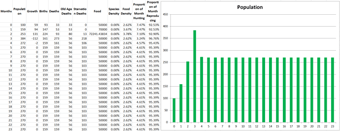
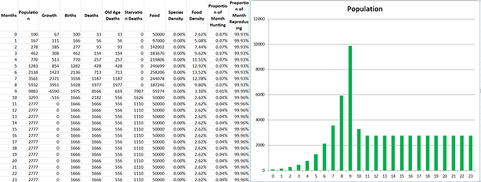
In the original scenario, the population stabilizes at 270 individuals. We’ve analyzed why it follows the pattern we see in the past part, but to recap: The population grows quickly at first due to an abundance of food, but then when shortage hits it stabilizes at a lower level where the rates of food consumption match the rate of food regeneration.
Simulation 1: Increased Mating Frequency
Starting Conditions
- Simulation Time = 24 months
- Modelus Specius
- Starting Population = 100
- Available Reproducers = 1.0
- Mating Frequency = 4/month
- Litter Size = 1
- Lifespan = 3 month
- Base Metabolism = 300 calories/month
- Swim Speed = 1cm/s
- Body Radius = 0.5cm
- Body Volume = 0.52cm^3
- Food
- Starting Amount = 50000
- Energy Yield = 1 calories
- Regeneration Rate = 50000/month
- Body Radius = 5cm
- Body Volume = 523.6cm^3
The cells of Modelus Specius have evolved special proteins that greatly accelerate the replicating process, causing the cells to double their original number 4x as quickly as before to produce offspring organisms through budding.
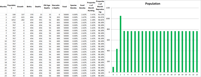
In this scenario the population stabilizes at 767. It’s interesting to consider why an increase in mating frequency led to such an increase in population. It also seems like Modelus Specius spends less time of the month hunting. I think the main reason why we see the increase in population is that increased mating frequency means more births to offset the number of deaths from old age and starvation. In fact you can see that every year the majority of the population dies of starvation (600 of the 767), but the surviving 167 have so many offspring that it keeps the species alive. This is a very interesting strategy that I had never even considered so far, and keep in mind how simple our model currently is! It’s crazy to see how it can already start producing these interesting interactions.
Simulation 2: Increased Litter Size
Starting Conditions
- Simulation Time = 24 months
- Modelus Specius
- Starting Population = 100
- Available Reproducers = 1.0
- Mating Frequency = 1/month
- Litter Size = 4
- Lifespan = 3 month
- Base Metabolism = 300 calories/month
- Swim Speed = 1cm/s
- Body Radius = 0.5cm
- Body Volume = 0.52cm^3
- Food
- Starting Amount = 50000
- Energy Yield = 1 calories
- Regeneration Rate = 50000/month
- Body Radius = 5cm
- Body Volume = 523.6cm^3
A mutation to the DNA for Modelus Specius’ budding has created the unique situation where it grows four buds simultaneously and then releases all of them, increasing the number of offspring produced per reproduction.
I ran the numbers on this and it produces the exact same outcome as the scenario above. At the moment litter size and mating frequency have effectively the same effect on the simulation.
Simulation 3: Lower Base Metabolism
Starting Conditions
- Simulation Time = 24 months
- Modelus Specius
- Starting Population = 100
- Available Reproducers = 1.0
- Mating Frequency = 1/month
- Litter Size = 1
- Lifespan = 3 month
- Base Metabolism = 150 calories/month
- Swim Speed = 1cm/s
- Body Radius = 0.5cm
- Body Volume = 0.52cm^3
- Food
- Starting Amount = 50000
- Energy Yield = 1 calories
- Regeneration Rate = 50000/month
- Body Radius = 5cm
- Body Volume = 523.6cm^3
The cells of Modelus Specius have evolved a more efficient method of spending energy to perform processes in the body, and as such only require half as much energy (5 calories per individual per day) for their base metabolism.
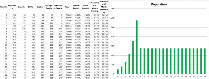
In this scenario the population stabilizes at 548. Since the population consumes less energy at the start, it takes longer for the food shortage to hit so we see the population peak on the 5th month instead of the 2nd. My guess for the increase in population over the standard simulation is that since each individual only requires half as much energy, they only spend half as long hunting (2% of their time instead of 4%) which means they can spend that extra 2% of their time reproducing. It ALSO is because of the fact that with half the base metabolism as before, the environment now produces enough energy to support double the population.
Simulation 4: Increased Swim Speed
Starting Conditions
- Simulation Time = 24 months
- Modelus Specius
- Starting Population = 100
- Available Reproducers = 1.0
- Mating Frequency = 1/month
- Litter Size = 1
- Lifespan = 3 month
- Base Metabolism = 300 calories/month
- Swim Speed = 10cm/s
- Body Radius = 0.5cm
- Body Volume = 0.52cm^3
- Food
- Starting Amount = 50000
- Energy Yield = 1 calories
- Regeneration Rate = 50000/month
- Body Radius = 5cm
- Body Volume = 523.6cm^3
Some cells on the edges of Modelus Specius have evolved some of their internal proteins into elastic fibres that can cause them to expand and contract at a greater range of motion. This allows the organism to undulate with wider motions and swim faster (from 1cm/s to 10cm/s).
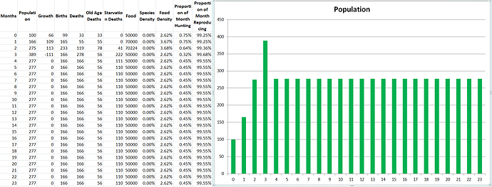
In this scenario the population stabilizes at 277 (remember standard simulation was 270). I think this tiny increase is because so little time was being spent hunting anyways, that increasing speed by 10x barely affects the overall population. Yes in the last simulation the less time spent hunting increased population, but remember it also involved less energy being consumed overall which greatly increased the OVERALL population that could be supported. Here the population cannot grow any larger because starvation rates will keep it in check.
Simulation 5: Higher Food Energy Yield
Starting Conditions
- Simulation Time = 24 months
- Modelus Specius
- Starting Population = 100
- Available Reproducers = 1.0
- Mating Frequency = 1/month
- Litter Size = 1
- Lifespan = 3 month
- Base Metabolism = 300 calories/month
- Swim Speed = 1cm/s
- Body Radius = 0.5cm
- Body Volume = 0.52cm^3
- Food
- Starting Amount = 50000
- Energy Yield = 10 calories
- Regeneration Rate = 50000/month
- Body Radius = 5cm
- Body Volume = 523.6cm^3
Chemical changes on the surface of the ocean have led to denser clouds of glucose floating in the oceans, containing 10x as much energy.
In this scenario, the population stabilizes at 2777. I know that this is technically not a mutation to the species but a change to the environment, but I wanted to try it too. We can see that increasing the energy yield of the food drastically affects the species’ population. It takes much longer for the food shortage to hit, so the population peaks on the 9th month instead of the 2nd. Also, each food cloud is so energy rich that each individual only needs to hunt 1 to receive all the energy they need for an entire month, drastically reducing the time they spend hunting. Since 50,000 units of food are produced every month, but the energy of that food has increased 10x, the environment can now support a much higher population with the energy it produces. For all these reasons (and maybe a few more I’m not thinking of), the population of Modelus Specius is effectively able to increase by 10x.
Final Results
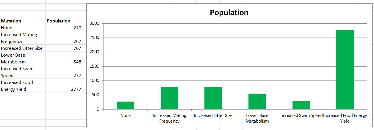
Now we can look at the final population achieved with each mutation.
Obviously the Increased Food Energy Yield had the greatest effect, but let’s pretend we are Auto-Evo and that is not an option. We would choose Increased Mating Frequency or Increased Litter Size as the mutation for Modelus Specius, since it produced the greatest increase in population size.
Also keep in mind that the “strength” of those different mutations depended a lot on the conditions of the environment. Since energy was so abundant, lower base metabolism and increased swim speed were not as effective as adaptations, whereas increased mating frequency or increased litter size allowed the species to rapidly grow its population and make greater use of the plentitude of energy in the environment. Perhaps if energy was much harder to come by, lower base metabolism and increased swim speed would have been much better adaptations!
I hope you guys found that interesting and that it helped give a sense of how the algorithm works and how it will ultimately be used to guide Auto-Evo. It definitely did whet my appetite for seeing evolution in action in the final game. I think these demo simulations will only get more and more interesting as we add more elements to the algorithm. Next time we’ll be back with the next part in the series!

