FOREWORD
After some thought and discussions on Discord, I’ve realized that this next part is actually mostly unnecessary. However, it’s worth discussing the parts of it that matter, so get ready for probably the shortest part of this series.
Part 4: Demography
As you can see, within just a few parts we’ve already quite rapidly created a rudimentary auto-evo algorithm, with traits like swimming speed, base metabolism, and mating frequency factoring into the survivability of species. I really like the approach we are taking because it feels like we are building the framework of the algorithm, and then filling in the details later. We will soon be ready to start introducing other species into the mix, but before we can do that there are two quick topics we must cover in their own parts.
The first is this part, on habitats and demography. How does where the species live affect its likelihood of interactions with other species? We have already factored in density, but there’s also other factors of the distribution of species in nature such as preferred habitats, habitat overlap, clustering, etc.
We will revisit other aspects of habitats again in the future, such as migrations, environmental conditions, territoriality, etc. For now though, we must simply consider where in the patch Modelus Specius is likely to live and how that affects its interactions with other actors in the patch.
We will be breaking down the following 2 assumptions from our list:
- Modelus Specius is a flat, tiny, simple, jelly-like organism that lives at the bottom of the ocean.
- Members of the species can instantly perceive food regardless of distance (Perception)
- Members of the species can completely consume the food and gain 100% of the energy. (Hunting/Metabolism)
- The species is equally distributed/dispersed across the world (Demographics)
- The planet is one giant ocean of equal pressure water that is equally accessible to the player (Geography/Terrain)
- Modelus Specius is the only species on the planet (Ecology)
- Members can reproduce as many times as they want, instantly, with no pregnancy/gestation period. (Reproduction)
- The species reproduces via asexual reproduction, spawning fully developed offspring that can themselves immediately begin reproducing. (Mating)
- The species does not change in physiology as they age (Aging/Ontogeny)
- The species is fully aquatic (Terrestriality)
- Members of the species are solitary and do not cooperate with other species members in any way. (Cooperation/Sociality)
- The species has no parental instincts, and will immediately abandon offspring (Parenting)
- The species is perfectly adapted to its environment and suffers no death or disease from environmental conditions (Environment)
Questions to Consider
When addressing these two assumptions, there are a few questions that are raised:
- What would a species’ habitat look like? Can it be assumed that a species occupies the whole patch? Or only parts of the patch?
- If they only occupy parts of the patch, how do we calculate overlap?
- Is the species evenly distributed across the entire habitat they occupy? Or are they clustered?
- Are there inaccessible zones of the patch? (Physical barriers, isolated bodies of water, pressure differences, other physiochemical differences)
Habitats
What would a species’ habitat look like? Can it be assumed that a species occupies the whole patch? Or only parts of the patch?
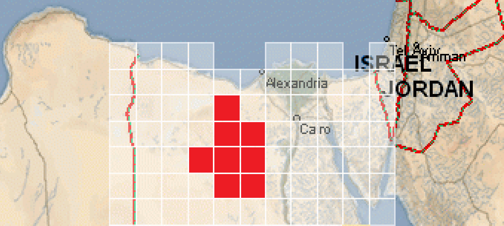
From the definition of a patch, we are going to assume that all species in a patch occupy all parts of that patch. Habitats thus will not be defined by what parts inside of a patch are occupied by the species, but rather which specific patches are occupied in the first place. For example, consider the following diagram:
A species of camels would have their habitat defined by the 8 Desert patches that they occupy. However, within those patches the camels would be assumed to live in the entire area/space. This concept will be explored more in Episode 2.
Patches will tend to be smaller and represent a piece of land or ocean or sky that has very similar living conditions all across, so this is a fair assumption to make.
Overlap
If they only occupy parts of the patch, how do we calculate overlap?
This question is irrelevant because of the answer to the first question. Since we are not assigning specific habitats inside of a patch, overlap is unnecessary because all species in a patch will ALWAYS overlap. Therefore overlap will be more in regards to whether 2 species live in the same patch, and how many patches they live together in. This is something to revisit in Episode 2.
Clustering
Is the species evenly distributed across the entire habitat they occupy? Or are they clustered?
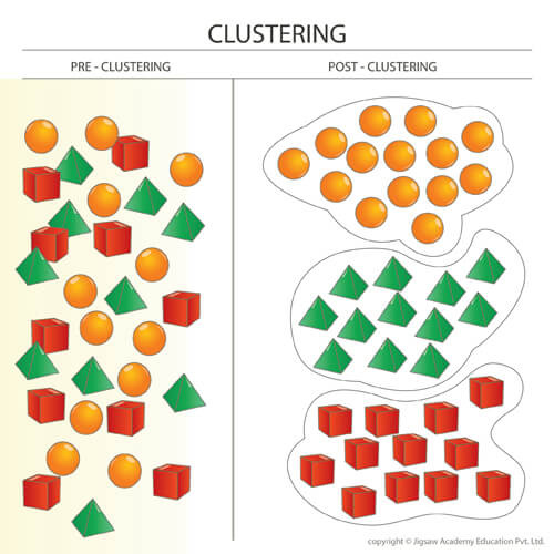
Here is an interesting point to consider. It might be difficult to imagine how clustering would affect demographics, so here’s a diagram to help illustrate the point.
Imagine a scenario with multiple species that fill up the entire patch, aka a case of high spatial density (remember that population density was renamed to spatial density). With even distribution, as seen on the left side, the average distance between any one species and the nearest member of another species is quite short, something we explored in part 3. When distribution is even, this is equivalent to minimal clustering (or a clustering value of 0).
When clustering is maximized (a clustering value of 1.0), all species are lumped into big groups. Notice how suddenly the average distance between any species member and a member from another species becomes much longer. For example the orange species members are now much further from the red species members.
So imagine you are a predator. Increased spatial density of your species and the prey species is a BENEFIT because it makes it more likely for a prey to be very nearby to you. Therefore, increased clustering diminishes the benefit of spatial density by grouping members of a species together, instead of allowing them to be mixed in. Another way of thinking about it: Increased density decreases the average distance to a prey, and increased clustering decreases the effect of density, therefore increased clustering increases the average distance to a prey.
On the flip side, when spatial density is low, clustering doesn’t really matter because there are fewer individuals (think of just 1 predator and 1 prey, clustering is irrelevant in such a case because there is no one to cluster with).
So this is the current equation for calculating the average distance between a predator and its prey, factoring in the spatial density of both species:
Distance per Hunt = (0.66 * Patch Length) * (1 - (4 * Predator Population Density * Prey Population Density)) - Predator Body Radius - Prey Body Radius
Now we’ll add in a term that diminishes the density term. First we calculating the Average Clustering between the two species, and then factor that into the overall equation:
Average Clustering = (Predator Clustering + Prey Clustering) / 2
Distance per Hunt = (0.66 * Patch Length) * (1 - (4 * Predator Population Density * Prey Population Density * (1 - Average Clustering))) - Predator Body Radius - Prey Body Radius
With the above equation, when density is high then high clustering can reduce its effect, but when density is low the level of clustering is irrelevant. Clustering can never actually make the average distance to a prey increase more than it normally would be, it can only reduce density’s effect of making it shorter.
NOTE: Clustering will be defined as a species trait. Why would a species ever evolve clustering? If you are a prey to many species, it will make it less likely for you to be found by predators since you can hide all your species members in a corner. Also, clustering will be necessary for cooperative social behaviours that we’ll introduce in a future part.
Inaccessible Zones
Are there inaccessible zones of the patch? (Physical barriers, isolated bodies of water, pressure differences, other physiochemical differences)
To this I would again say no due to the definition of a patch. A patch is defined as a contiguous space with common physicochemical features, so if there was a barrier that would define a separate patch. Thus we don’t need to consider this.
Filling up the Oceans
Finally, before we can close, there’s one more point to consider. The algorithm actually currently has no limit on the number of organisms that can exist in the patch. Modelus Specius could theoretically have millions of offspring and fill the oceans of the world multiple times over (if there was enough food). We should introduce a limitation in terms of physical space to prevent this from ever occurring.
We will do this by limiting births. If the number of births is ever going to produce more offspring than can physically fit in the patch, we will just limit it to what can physically fit. I’ll skip showing the math behind this because I think it makes sense already, but if someone wants to see the equations for it let me know.
Demos
There will be no demos this part, since the changes were so minor and barely visible in the results. I did notice though that increasing clustering did lead to either more time spent hunting, or lower overall populations for Modelus Specius because of less free time to reproduce.
As compensation for this less eventful part, the next part will be coming out pretty soon!
Summary
New Performance Stats
None
New Traits
Clustering
Topics for Discussion
All comments and feedback are welcome!

