Nick's Auto-Evo Algorithm (Episode 1)

[tjwhale]

I am very inspired by KSP too, that’s what I would like to push towards, a lego like set of building tools which the player uses to overcome complex and challenging scientific problems in a fun way.

@NickTheNick

Worst case scenario, it’s much easier to take a system that is too complex and simplify it, than to take a simple model and make it deeper and more complex.

I am not sure about this, I think the opposite might be true. However as with many things doing a bunch of experiments is a good way of proceeding.

Also on the issue of complexity I think it shouldn’t be so hard to find enough. Even simple games like the prisoners dilemma become complex and interesting when played iteratively between multiple agents with different strategies.

@NickTheNick

I do personally enjoy making the episodes and being able to play with the simulation.

Awesome

[NickTheNick]

Yeah I think experimentation is our major benefit. Since we are building it iteratively and from such a simple original framework, we can keep track of the entire algorithm as we build it and intervene if it starts to get too chaotic or complex at any point.

[NickTheNick]

Part 3.1: Simulation Demos

As I mentioned in the last part, we’ll now do a series of demos with different parameters to better explore the system we’ve created so far, and see how changes to traits affect the population of the species. Hopefully it can also give us a taste for what the finished Auto-Evo system will feel like in the game!

Before we begin, however, running these simulations was helpful since it helped me find to flaws with the algorithm’s design. Firstly, I realized that people should die of old age at the end of the timestep, not the beginning. If the lifespan for a species is 1 month or lower, the entire population will die of old age before they get to do anything, which doesn’t make any sense. This change doesn’t change anything other than fixing that problem, and I’m not really sure why I didn’t think of this earlier. Here is what the new Life Cycle Diagram looks like:

Which much more closely resembles the typical lifespan of an organism (birth, survival, reproduction, death from old age).

Secondly, I’ve renamed the Population Density performance stat to now be called Spatial Population Density, since it’s actually a measure of what ratio of space the population occupies. This is so that Population Density can refer to its actual meaning of a number of individuals per unit of area or unit of volume.

Finally, to make things more interesting, I’ve tweaked some of the stats of the Standard Simulation to make life more difficult for the species. Then the following changes will almost be an experiment to see which is the best mutation. In fact we’re basically playing as the Auto-Evo system here, since the system will assign random mutations to a species and see which one best increases its survival. First, let’s begin with our baseline, the Standard Simulation.

Simulation 0: Standard Simulation

Starting Conditions

• Simulation Time = 24 months
• Modelus Specius
  • Starting Population = 100
  • Available Reproducers = 1.0
  • Mating Frequency = 1/month
  • Litter Size = 1
  • Lifespan = 3 month
  • Base Metabolism = 300 calories/month
  • Swim Speed = 1cm/s
  • Body Radius = 0.5cm
  • Body Volume = 0.52cm^3
• Food
  • Starting Amount = 50000
  • Energy Yield = 1 calories
  • Regeneration Rate = 50000/month
  • Body Radius = 5cm
  • Body Volume = 523.6cm^3

In the original scenario, the population stabilizes at 270 individuals. We’ve analyzed why it follows the pattern we see in the past part, but to recap: The population grows quickly at first due to an abundance of food, but then when shortage hits it stabilizes at a lower level where the rates of food consumption match the rate of food regeneration.

Simulation 1: Increased Mating Frequency

Starting Conditions

• Simulation Time = 24 months
• Modelus Specius
  • Starting Population = 100
  • Available Reproducers = 1.0
  • Mating Frequency = 4/month
  • Litter Size = 1
  • Lifespan = 3 month
  • Base Metabolism = 300 calories/month
  • Swim Speed = 1cm/s
  • Body Radius = 0.5cm
  • Body Volume = 0.52cm^3
• Food
  • Starting Amount = 50000
  • Energy Yield = 1 calories
  • Regeneration Rate = 50000/month
  • Body Radius = 5cm
  • Body Volume = 523.6cm^3

The cells of Modelus Specius have evolved special proteins that greatly accelerate the replicating process, causing the cells to double their original number 4x as quickly as before to produce offspring organisms through budding.

In this scenario the population stabilizes at 767. It’s interesting to consider why an increase in mating frequency led to such an increase in population. It also seems like Modelus Specius spends less time of the month hunting. I think the main reason why we see the increase in population is that increased mating frequency means more births to offset the number of deaths from old age and starvation. In fact you can see that every year the majority of the population dies of starvation (600 of the 767), but the surviving 167 have so many offspring that it keeps the species alive. This is a very interesting strategy that I had never even considered so far, and keep in mind how simple our model currently is! It’s crazy to see how it can already start producing these interesting interactions.

Simulation 2: Increased Litter Size

Starting Conditions

• Simulation Time = 24 months
• Modelus Specius
  • Starting Population = 100
  • Available Reproducers = 1.0
  • Mating Frequency = 1/month
  • Litter Size = 4
  • Lifespan = 3 month
  • Base Metabolism = 300 calories/month
  • Swim Speed = 1cm/s
  • Body Radius = 0.5cm
  • Body Volume = 0.52cm^3
• Food
  • Starting Amount = 50000
  • Energy Yield = 1 calories
  • Regeneration Rate = 50000/month
  • Body Radius = 5cm
  • Body Volume = 523.6cm^3

A mutation to the DNA for Modelus Specius’ budding has created the unique situation where it grows four buds simultaneously and then releases all of them, increasing the number of offspring produced per reproduction.

I ran the numbers on this and it produces the exact same outcome as the scenario above. At the moment litter size and mating frequency have effectively the same effect on the simulation.

Simulation 3: Lower Base Metabolism

Starting Conditions

• Simulation Time = 24 months
• Modelus Specius
  • Starting Population = 100
  • Available Reproducers = 1.0
  • Mating Frequency = 1/month
  • Litter Size = 1
  • Lifespan = 3 month
  • Base Metabolism = 150 calories/month
  • Swim Speed = 1cm/s
  • Body Radius = 0.5cm
  • Body Volume = 0.52cm^3
• Food
  • Starting Amount = 50000
  • Energy Yield = 1 calories
  • Regeneration Rate = 50000/month
  • Body Radius = 5cm
  • Body Volume = 523.6cm^3

The cells of Modelus Specius have evolved a more efficient method of spending energy to perform processes in the body, and as such only require half as much energy (5 calories per individual per day) for their base metabolism.

In this scenario the population stabilizes at 548. Since the population consumes less energy at the start, it takes longer for the food shortage to hit so we see the population peak on the 5th month instead of the 2nd. My guess for the increase in population over the standard simulation is that since each individual only requires half as much energy, they only spend half as long hunting (2% of their time instead of 4%) which means they can spend that extra 2% of their time reproducing. It ALSO is because of the fact that with half the base metabolism as before, the environment now produces enough energy to support double the population.

Simulation 4: Increased Swim Speed

Starting Conditions

• Simulation Time = 24 months
• Modelus Specius
  • Starting Population = 100
  • Available Reproducers = 1.0
  • Mating Frequency = 1/month
  • Litter Size = 1
  • Lifespan = 3 month
  • Base Metabolism = 300 calories/month
  • Swim Speed = 10cm/s
  • Body Radius = 0.5cm
  • Body Volume = 0.52cm^3
• Food
  • Starting Amount = 50000
  • Energy Yield = 1 calories
  • Regeneration Rate = 50000/month
  • Body Radius = 5cm
  • Body Volume = 523.6cm^3

Some cells on the edges of Modelus Specius have evolved some of their internal proteins into elastic fibres that can cause them to expand and contract at a greater range of motion. This allows the organism to undulate with wider motions and swim faster (from 1cm/s to 10cm/s).

In this scenario the population stabilizes at 277 (remember standard simulation was 270). I think this tiny increase is because so little time was being spent hunting anyways, that increasing speed by 10x barely affects the overall population. Yes in the last simulation the less time spent hunting increased population, but remember it also involved less energy being consumed overall which greatly increased the OVERALL population that could be supported. Here the population cannot grow any larger because starvation rates will keep it in check.

Simulation 5: Higher Food Energy Yield

Starting Conditions

• Simulation Time = 24 months
• Modelus Specius
  • Starting Population = 100
  • Available Reproducers = 1.0
  • Mating Frequency = 1/month
  • Litter Size = 1
  • Lifespan = 3 month
  • Base Metabolism = 300 calories/month
  • Swim Speed = 1cm/s
  • Body Radius = 0.5cm
  • Body Volume = 0.52cm^3
• Food
  • Starting Amount = 50000
  • Energy Yield = 10 calories
  • Regeneration Rate = 50000/month
  • Body Radius = 5cm
  • Body Volume = 523.6cm^3

Chemical changes on the surface of the ocean have led to denser clouds of glucose floating in the oceans, containing 10x as much energy.

In this scenario, the population stabilizes at 2777. I know that this is technically not a mutation to the species but a change to the environment, but I wanted to try it too. We can see that increasing the energy yield of the food drastically affects the species’ population. It takes much longer for the food shortage to hit, so the population peaks on the 9th month instead of the 2nd. Also, each food cloud is so energy rich that each individual only needs to hunt 1 to receive all the energy they need for an entire month, drastically reducing the time they spend hunting. Since 50,000 units of food are produced every month, but the energy of that food has increased 10x, the environment can now support a much higher population with the energy it produces. For all these reasons (and maybe a few more I’m not thinking of), the population of Modelus Specius is effectively able to increase by 10x.

Final Results

Now we can look at the final population achieved with each mutation.

Obviously the Increased Food Energy Yield had the greatest effect, but let’s pretend we are Auto-Evo and that is not an option. We would choose Increased Mating Frequency or Increased Litter Size as the mutation for Modelus Specius, since it produced the greatest increase in population size.

Also keep in mind that the “strength” of those different mutations depended a lot on the conditions of the environment. Since energy was so abundant, lower base metabolism and increased swim speed were not as effective as adaptations, whereas increased mating frequency or increased litter size allowed the species to rapidly grow its population and make greater use of the plentitude of energy in the environment. Perhaps if energy was much harder to come by, lower base metabolism and increased swim speed would have been much better adaptations!

I hope you guys found that interesting and that it helped give a sense of how the algorithm works and how it will ultimately be used to guide Auto-Evo. It definitely did whet my appetite for seeing evolution in action in the final game. I think these demo simulations will only get more and more interesting as we add more elements to the algorithm. Next time we’ll be back with the next part in the series!

[NickTheNick]

FOREWORD
After some thought and discussions on Discord, I’ve realized that this next part is actually mostly unnecessary. However, it’s worth discussing the parts of it that matter, so get ready for probably the shortest part of this series.

Part 4: Demography

As you can see, within just a few parts we’ve already quite rapidly created a rudimentary auto-evo algorithm, with traits like swimming speed, base metabolism, and mating frequency factoring into the survivability of species. I really like the approach we are taking because it feels like we are building the framework of the algorithm, and then filling in the details later. We will soon be ready to start introducing other species into the mix, but before we can do that there are two quick topics we must cover in their own parts.

The first is this part, on habitats and demography. How does where the species live affect its likelihood of interactions with other species? We have already factored in density, but there’s also other factors of the distribution of species in nature such as preferred habitats, habitat overlap, clustering, etc.

We will revisit other aspects of habitats again in the future, such as migrations, environmental conditions, territoriality, etc. For now though, we must simply consider where in the patch Modelus Specius is likely to live and how that affects its interactions with other actors in the patch.

We will be breaking down the following 2 assumptions from our list:

• Modelus Specius is a flat, tiny, simple, jelly-like organism that lives at the bottom of the ocean.
• Members of the species can instantly perceive food regardless of distance (Perception)
• Members of the species can completely consume the food and gain 100% of the energy. (Hunting/Metabolism)
• The species is equally distributed/dispersed across the world (Demographics)
• The planet is one giant ocean of equal pressure water that is equally accessible to the player (Geography/Terrain)
• Modelus Specius is the only species on the planet (Ecology)
• Members can reproduce as many times as they want, instantly, with no pregnancy/gestation period. (Reproduction)
• The species reproduces via asexual reproduction, spawning fully developed offspring that can themselves immediately begin reproducing. (Mating)
• The species does not change in physiology as they age (Aging/Ontogeny)
• The species is fully aquatic (Terrestriality)
• Members of the species are solitary and do not cooperate with other species members in any way. (Cooperation/Sociality)
• The species has no parental instincts, and will immediately abandon offspring (Parenting)
• The species is perfectly adapted to its environment and suffers no death or disease from environmental conditions (Environment)

Questions to Consider

When addressing these two assumptions, there are a few questions that are raised:

• What would a species’ habitat look like? Can it be assumed that a species occupies the whole patch? Or only parts of the patch?
• If they only occupy parts of the patch, how do we calculate overlap?
• Is the species evenly distributed across the entire habitat they occupy? Or are they clustered?
• Are there inaccessible zones of the patch? (Physical barriers, isolated bodies of water, pressure differences, other physiochemical differences)

Habitats

What would a species’ habitat look like? Can it be assumed that a species occupies the whole patch? Or only parts of the patch?

From the definition of a patch, we are going to assume that all species in a patch occupy all parts of that patch. Habitats thus will not be defined by what parts inside of a patch are occupied by the species, but rather which specific patches are occupied in the first place. For example, consider the following diagram:

A species of camels would have their habitat defined by the 8 Desert patches that they occupy. However, within those patches the camels would be assumed to live in the entire area/space. This concept will be explored more in Episode 2.

Patches will tend to be smaller and represent a piece of land or ocean or sky that has very similar living conditions all across, so this is a fair assumption to make.

Overlap

If they only occupy parts of the patch, how do we calculate overlap?

This question is irrelevant because of the answer to the first question. Since we are not assigning specific habitats inside of a patch, overlap is unnecessary because all species in a patch will ALWAYS overlap. Therefore overlap will be more in regards to whether 2 species live in the same patch, and how many patches they live together in. This is something to revisit in Episode 2.

Clustering

Is the species evenly distributed across the entire habitat they occupy? Or are they clustered?

Here is an interesting point to consider. It might be difficult to imagine how clustering would affect demographics, so here’s a diagram to help illustrate the point.

Imagine a scenario with multiple species that fill up the entire patch, aka a case of high spatial density (remember that population density was renamed to spatial density). With even distribution, as seen on the left side, the average distance between any one species and the nearest member of another species is quite short, something we explored in part 3. When distribution is even, this is equivalent to minimal clustering (or a clustering value of 0).

When clustering is maximized (a clustering value of 1.0), all species are lumped into big groups. Notice how suddenly the average distance between any species member and a member from another species becomes much longer. For example the orange species members are now much further from the red species members.

So imagine you are a predator. Increased spatial density of your species and the prey species is a BENEFIT because it makes it more likely for a prey to be very nearby to you. Therefore, increased clustering diminishes the benefit of spatial density by grouping members of a species together, instead of allowing them to be mixed in. Another way of thinking about it: Increased density decreases the average distance to a prey, and increased clustering decreases the effect of density, therefore increased clustering increases the average distance to a prey.

On the flip side, when spatial density is low, clustering doesn’t really matter because there are fewer individuals (think of just 1 predator and 1 prey, clustering is irrelevant in such a case because there is no one to cluster with).

So this is the current equation for calculating the average distance between a predator and its prey, factoring in the spatial density of both species:

Distance per Hunt = (0.66 * Patch Length) * (1 - (4 * Predator Population Density * Prey Population Density)) - Predator Body Radius - Prey Body Radius

Now we’ll add in a term that diminishes the density term. First we calculating the Average Clustering between the two species, and then factor that into the overall equation:

Average Clustering = (Predator Clustering + Prey Clustering) / 2
Distance per Hunt = (0.66 * Patch Length) * (1 - (4 * Predator Population Density * Prey Population Density * (1 - Average Clustering))) - Predator Body Radius - Prey Body Radius

With the above equation, when density is high then high clustering can reduce its effect, but when density is low the level of clustering is irrelevant. Clustering can never actually make the average distance to a prey increase more than it normally would be, it can only reduce density’s effect of making it shorter.

NOTE: Clustering will be defined as a species trait. Why would a species ever evolve clustering? If you are a prey to many species, it will make it less likely for you to be found by predators since you can hide all your species members in a corner. Also, clustering will be necessary for cooperative social behaviours that we’ll introduce in a future part.

Inaccessible Zones

Are there inaccessible zones of the patch? (Physical barriers, isolated bodies of water, pressure differences, other physiochemical differences)

To this I would again say no due to the definition of a patch. A patch is defined as a contiguous space with common physicochemical features, so if there was a barrier that would define a separate patch. Thus we don’t need to consider this.

Filling up the Oceans

Finally, before we can close, there’s one more point to consider. The algorithm actually currently has no limit on the number of organisms that can exist in the patch. Modelus Specius could theoretically have millions of offspring and fill the oceans of the world multiple times over (if there was enough food). We should introduce a limitation in terms of physical space to prevent this from ever occurring.

We will do this by limiting births. If the number of births is ever going to produce more offspring than can physically fit in the patch, we will just limit it to what can physically fit. I’ll skip showing the math behind this because I think it makes sense already, but if someone wants to see the equations for it let me know.

Demos

There will be no demos this part, since the changes were so minor and barely visible in the results. I did notice though that increasing clustering did lead to either more time spent hunting, or lower overall populations for Modelus Specius because of less free time to reproduce.

As compensation for this less eventful part, the next part will be coming out pretty soon!

---

Summary

New Performance Stats
None

New Traits
Clustering

Topics for Discussion
All comments and feedback are welcome!

[NickTheNick]

I realized I made a mistake with the corrected diagram at the top of this post. It should actually look like this:

In the updated algorithm, the first thing that happens is that the script determines what fraction of the population dies from starvation and kills them off first. Then of the remaining population, it determines how many offspring were birthed. Before it adds the births, it also kills off any of the population members who die from old age. Therefore births and old age deaths occur sort of in parallel.

Anyways, just wanted to make that clear and I’ll go back and fix the original post later. The next part will be coming up soon! Feel free to leave any suggestions or feedback you have on the series so far.

[NickTheNick]

Part 5: Hydrodynamics and Swimming

Yes we have a stat for movement speed now, but it’s a generic stat that is not tied to the organism’s body or the environment in any way. In this part we will look at the hydrodynamics of swimming and how to make movement speed realistically determined. There are no specific assumptions from our list that we are breaking down, instead we are just adding detail to the movement calculations from Part 3. Let’s find out how to make a creature’s swimming speed depend on its size, shape, and surroundings.

Undulation

Modelus Specius is a simple, spherical creature comprised of simple tissue. We’ll assume that this simple tissue has basic abilities to perform various tasks, such as in this case contracting to act like a muscle. We’ll classify Modelus Specius as using the type of swimming referred to as undulation, meaning it flexes the sides of its spherical body back and forth to propel itself forward. Thus we’ll say only the tissue on the sides of its body are contributing their force towards the swimming motion.

It’s hard to imagine how a solid sphere would use undulation, so imagine it as similar to the motion used by jellyfish (except that there is no hollow cavity or tentacles in the bottom).

Online, it says that the fastest recorded speed of a jellyfish is 8 kph. Dividing by ten I think gives us a more realistic top speed for small and simple jellies that are similar to Modelus Specius, so a top speed of 0.8 kph or 0.2 m/s. Now, for the next step, let’s take a look at Forces.

Force

Force is a simple concept in physics. It’s basically an interaction or energy that changes the motion of an object. When an object experiences a net force in a direction, it accelerates in that direction. When an object experiences no net forces in a direction, it maintains its motion in that direction (which could be maintaining its current speed without decelerating, or it could be being completely motionless). Keep in mind that accelerating in one direction (such as backwards) is the same as decelerating in the opposite direction (forwards). Why “net” force by the way? Because you can have multiple forces that act in opposing directions, but the ones that are greater will determine how the object’s motion changes.

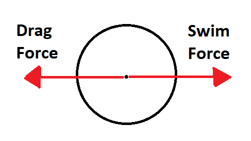
For Modelus Specius’ swimming, we will consider its motion as an interplay of two forces: The “thrust” or “swim” force that the organism produces to propel itself forwards, and the drag force of water pushing back against it as it swims. We can visually display these using a diagram common in physics, a free-body diagram

Drag Force

At top speed, the swim force and the drag force will perfectly balance each other out, resulting in top speed being achieved and no more forward acceleration. Why is this the case? Because when you first start swimming, your Swim Force greatly outweighs your Drag Force. However, Drag Force increases with your speed, so as you speed up your Drag Force increased but your Swim Force stays the same. Eventually your Drag Forces reaches the value of your Swim Force, and that’s when you hit top speed and stop accelerating.

We already know the top speed of the Modelus Specius, which we’ve estimated at 0.2 m/s. But what if the ocean’s temperature changed and made water more resistant to swimming (higher drag)? What if Modelus Specius’ size got larger and less hydrodynamically shaped? Since drag force can vary so much, we should use our estimate of 0.2 m/s top speed to find the actual Swim Force produced by the jellyfish.

To find the Swim Force, we will find the Drag Force and know that by definition the Swim Force has to be the same value. Drag Force can be calculated using the following equation:

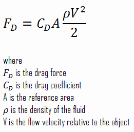
Let’s break this equation down variable by variable to see how drag will be calculated in Thrive.

Relative Flow Velocity

This refers to the difference of velocity (remember that velocity is just a physics term for speed with a direction) between the fluid and the object.

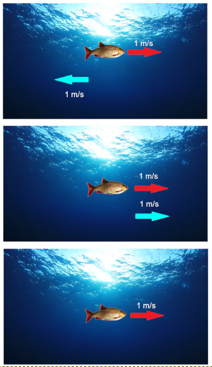
If the fluid flows in the opposite direction to the organism’s motion, then you add the velocities to find the relative velocity. If flowing in the same direction like the 2nd panel, you subtract them (if you and the water are both moving the same way, it feels like you’re not moving). If the water is motionless, you only consider the velocity of the organism. Okay, simple enough, but this brings us to a dilemma.

---

The Dilemma

Now obviously ocean currents are a very real phenomenon that play a big role in life, but I simply cannot imagine how to make an algorithm that takes into account the role of water currents, especially when most of the values being used are averages. Water currents flow in different directions at different speeds all over the ocean. Do we just take an average direction and average speed for the entire patch’s water current?

Okay, say we do that, how do we factor that into the algorithm? Do we apply that to the speed of the organism when he is hunting? How do we know when the water current is flowing in the same direction as the movement? In the opposite direction? How do we know when it’s flowing at a 30 degree angle from the organism’s motion. We could theoretically get an “average direction” for all hunts, but how would that be calculated? We’d have to get an average position for the predator population, and an average position for the prey population. And keeping track of the positions of objects in the patch opens a WHOLE new can of worms…

---

There are two possible solutions I see to this problem:

1. Completely ignore ocean currents and always assume the fluid’s velocity is 0.
2. Completely ignore ocean currents within a patch, but consider ocean currents between patches.

Ignoring Ocean Currents

This is a simple solution that makes it so that we always only consider the velocity of the organism.

Ocean Currents Between Patches

In this scenario, you do the same as in the first solution, but instead you track ocean currents between patches. This means that ocean currents can affect things like migrations between patches, or even moving to another patch to hunt (if that is intended to be possible), but not any interactions within a patch. I feel like this solution doesn’t sacrifice too much realism since ocean currents play a more important role on the larger scale (between patches) than the smaller scale (within patches).

For our purposes, we will proceed using the 2nd solution, which means the relative fluid velocity is equal to the velocity of the organism, which is 0.2 m/s. This gives us so far:

Drag Force = 0.2^2

Density of the Fluid

Next we must consider the density of the ocean. The density of ocean water on the surface is 1027 kg/m^3. As you go deeper, the density of seawater increases. However, it increases at different rates depending on what latitude you are at. Seawater at latitudes of around 30-40 degrees south (a region called the Pycnocline) follow this pattern:

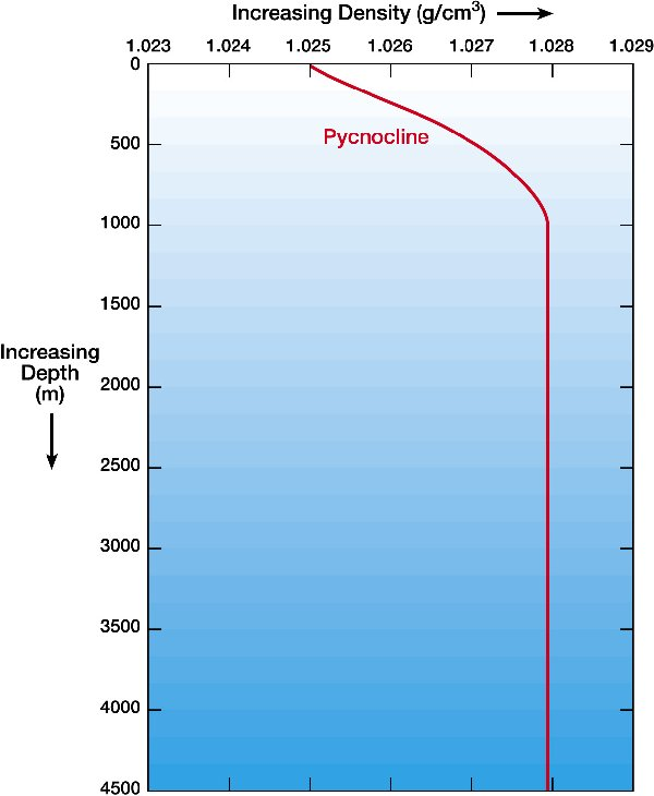
Modelus Specius lives at the bottom of the ocean, so let’s say the depth of the patch is 4000m. Assuming similar conditions to Earth at 30-40 degrees south, this gives us a density of 1028 kg/m^3. This means drag force is now:

Drag Force = 1028 * 0.2^2

We can simplify this and divide it by 2 (to get rid of the fraction in the formula) to get:

Drag Force = 20.56

Reference Area

When you swim into a certain direction, even though you are a 3D shape you are presenting a 2D profile or “silhouette” to the water. This “side” or “face” depends on which side you swim with, aka where is your front. Since Modelus Specius is a sphere, the frontal surface area is just a circle. In fact for a sphere any direction you look at it its 2D profile is just an equally shaped circle. Using the radius of Modelus Specius which we earlier defined as 0.5 cm, that gives us a circle area of 0.000079‬ m^2. This gives us:

Drag Force = 20.56 * 0.000079<U+202C> = 0.0016

Drag Coefficient

The drag coefficient is a value that takes into account the shape and texture of the object for how much drag it experiences. Many tests have already been done to find the Drag Coefficients for many reference shapes:

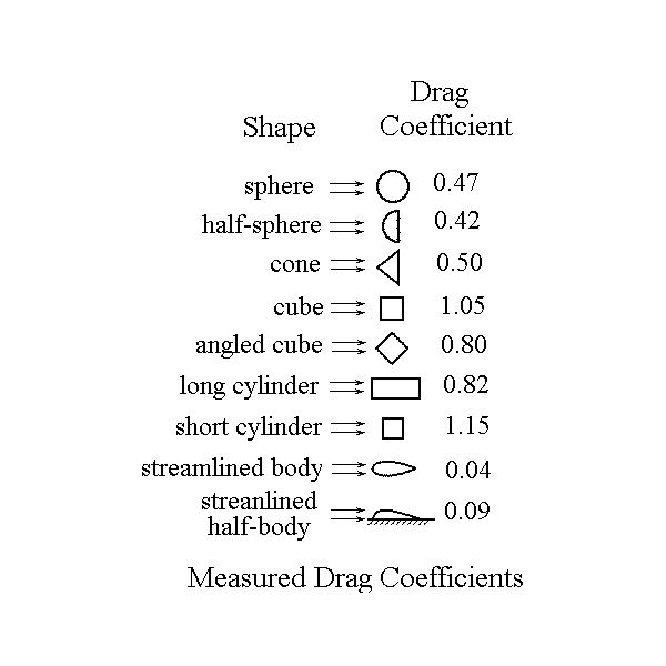
The Organism Editor will look at any species and assign the nearest approximation of drag coefficient based on what shape the front-side is closest to. Evolutions to skin (like hydrodynamically shaped scales) can increase or reduce the drag coefficient. Since Modelus Specius is a solid sphere, we’ll use the drag coefficient of 0.47.

Drag Force = 0.0016 * 0.47 = 0.00076

And that’s it! Our Drag Force is 0.00076 Newtons (the unit for force, also shortened to N). This means Modelus Specius must generate 0.00076 N of Swim Force.

Swim Force

When a muscle flexes, it produces a certain amount of force based off of the cross-sectional area of the muscle. Therefore if you know the area of the muscle, and since we know the force produced per area, you know the force the whole area can produce. Well for Modelus Specius it’s backwards, since we know the total force it can produce, and the total area involved in undulation, we can work backwards to find the force produced per area.

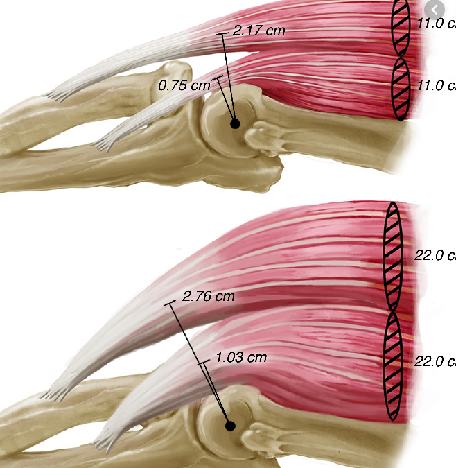
An example of cross-sectional area of human muscles.

A total of 0.00076N of force is being produced to swim when at top speed. The cross-sectional area of Modelus Specius is 0.000079‬ m^2. However, for realism’s purposes I would say that perhaps only 50% of the cells in the sphere are flexing and unflexing to produce the swimming motion, so that means half of that area so 0.000039 m^2. This gives a force per area of 19.5 N/m^2. Human muscle has a force per area of 350000 N/m^2. Yes, a lot more, but humans have also had millions of years to evolve their muscles to become incredibly efficient, whereas Modelus Specius is a very primitive species with very simple muscle fiber cells.

Updating the Algorithm

So now we have some values that we can put into the algorithm. Muscle Area (the area of cells involved in undulation), and Muscle Strength (the Newtons produced per area of the muscle). An organism uses these to produce Swim Force. Swim Force is then compared to the Drag Force caused by the environment, and the result determines the top speed of the organism.

One assumption this is making is that the organism will accelerate so quickly to its top speed that we can just use the top speed for its hunting speed, and ignore the time spent accelerating. For now we will have to make this assumption for simplicity’s sake, but in the future we can revisit this to try to flesh it out.

Demo

Running the updated algorithm gives us results very similar to Parts 4 and 3:

Starting Conditions

• Simulation Time = 24 months
• Modelus Specius
  • Starting Population = 100
  • Available Reproducers = 1.0
  • Mating Frequency = 1/month
  • Litter Size = 1
  • Lifespan = 3 months
  • Base Metabolism = 300 calories/month
  • Clustering = 0
  • Locomotion = Undulation
    • Muscle Area = 0.000039 m^2
    • Muscle Strength = 19.5 N/m^2
    • Drag Coefficient = 0.47
    • Frontal Surface Area = 0.000079 m^2
    • Swim Speed = 20cm/s (Derived from above above traits)
  • Body Radius = 0.5cm
  • Body Volume = 0.52cm^3
• Food
  Starting Amount = 50000
  Energy Yield = 1 calories
  Regeneration Rate = 50000/month
  Body Radius = 5cm
  Body Volume = 523.6cm^3

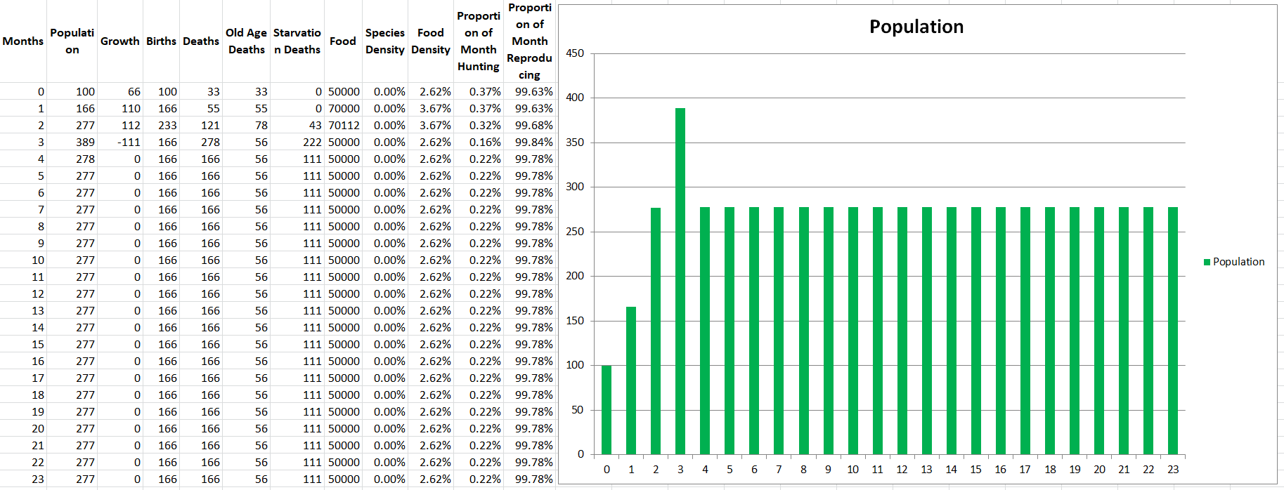
The population stabilizes around 277. The reason not much changed is that many of the changes we’ve made were under the hood, supporting more advanced interactions with other species and the environment in future parts. For example, we can now make environmental changes to the density of the oceans, or evolutionary changes to Modelus Specius’ body, and it will change the speed of its swimming. Something that did change though is that the speed of Modelus Specius is now around 20cm/s instead of 1cm/s, which has reduced the time they spend hunting every month to even less (0.22%).

Glad to be done with this pretty technical and not very rewarding part. Next time, we will finally, finally add in the main ingredient of evolution that we all love… Other species!

---

Summary

New Performance Stats
None

New Traits
Locomotion Type
Muscle Area (Swimming)
Muscle Strength (Swimming)
Coefficient of Drag
Frontal Surface Area

Topics for Discussion

• How do we model ocean currents?

[NickTheNick]

FOREWORD:

The addition of new species warranted some big changes to the algorithm’s code. Not only does Auto-Evo now have to loop through several species to run calculations every month, it also introduces new “race” mechanics to see who gets food first. These new features were much more complicated than I originally anticipated, and I basically learned the hard way why it’s so important to organize your code. I had to do an overhaul of the code to make it cleaner and more organized to add in the new features. I also had to greatly increase how much data was being displayed in the final reports to make them show a lot more information and use them for bugfixing. This way we can see much more detail into what is happening month by month and use it to debug the algorithm whenever I make a mistake (which I made a lot of when implementing these new features). There may have to be a part or two after this for bugfixing of the script if I catch any more. Anyways, all the major bugs have hopefully been ironed out, so time to showcase the next part!

Part 6: Competition

So far in the series, we’ve created a single species that eats, swims, reproduces, and inhabits certain parts of the patch based off density and clustering. But that’s not how evolution works, with just a single species. Evolution pits multiple species against each other! I think it’s time to start adding in some competition!

In this part we will be removing the following assumption from our list of assumptions:

• Modelus Specius is a flat, tiny, simple, jelly-like organism that lives at the bottom of the ocean.
• Members of the species can instantly perceive food regardless of distance (Perception)
• Members of the species can completely consume the food and gain 100% of the energy. (Hunting/Metabolism)
• Modelus Specius is the only species on the planet (Ecology)
• Members can reproduce as many times as they want, instantly, with no pregnancy/gestation period. (Reproduction)
• The species reproduces via asexual reproduction, spawning fully developed offspring that can themselves immediately begin reproducing. (Mating)
• The species does not change in physiology as they age (Aging/Ontogeny)
• The species is fully aquatic (Terrestriality)
• Members of the species are solitary and do not cooperate with other species members in any way. (Cooperation/Sociality)
• The species has no parental instincts, and will immediately abandon offspring (Parenting)
• The species is perfectly adapted to its environment and suffers no death or disease from environmental conditions (Environment)

We will start by adding one additional species to the environment. This species will have the exact same stats as Modelus Specius and feed on the same floating clouds of glucose. At the moment this is effectively equivalent to doubling the starting population of Modelus Specius, since they are both evenly matched. However instead of reaching an equilibrium with all of the population being in Modelus Specius, it will evenly split between the two species. After updating the algorithm, we’ll differ the stats of Species B to see if the environment reaches an equilibrium between the two species.

Then, once we have ironed out all the features of having two unique species in the environment, we will add two more species, and they will be given unique stats as well. Our goal is to create a simple environment of different species, that will serve as the foundation for the work we do in the future parts.

Also before we start, I tweaked some of the numbers of Modelus Specius to produce some more realistic outcomes for some of the statistics. Now the fraction spent hunting every month usually comes out closer to 30% of the month rather than 0.7%.

Summary of the changes

• Mating frequency was reduced by 50%
• Lifespan was increased to 12 months
• Base Metabolism was increased to 100 calories a day
• Muscle Strength reduced to 2.5N/m^2 (making the typical speed 7cm/s)

New Definitions

One more thing before we start the algorithm, it’s important to clarify the meaning of some terms I’ve been throwing around lately. I’ll add all of these entries to the glossary:

1. Generation: A generation refers to a “turn” in the game. For example, when you start the game you are playing on the first generation of your species. After reproducing, entering the editor, and a timestep passing, you resume play in the 2nd generation. Technically, yes, you could say that there’s thousands of generations that would’ve occurred in the thousands of years that passed during the timestep, but for the game’s purposes we call the time after each editor session a new “generation”.
2. Timestep: The time between generations is called the timestep. When a player enters the editor, does his stuff, and then returns to the game, the game fast forwards thousands or millions of years to represent the evolution that took place. That’s called a timestep. Every time the player reproduces and enters the editor, another timestep passes. Timestep just refers to the time that passed.
3. Simulation Step: This simply refers to the unit of time for simulation for the population algorithm. At the moment, this is one month. This means that all the calculations are run over the course of a month, and then repeated for however many months that we want the simulation to go for.

If there are any questions or suggestions about these definitions let me know. Anyways, on to the calculations!

Order of Calculations

One point I’ve been bringing up a lot is that the order of calculations is very important… Well it’s time to bring it up again! We are now going to have several species running inside the simulation at once, so the order of calculation is critical for decisions such as who gets first access to food.

Turn Order

My original idea was to use a “Turn Order” to handle the multiple species. This is because of the way the algorithm is designed, where we calculate the population change of one species at a time over one month, and then repeat that however many months. At the end of a generation, the game would randomly pick a turn order for all the available species, and then every month it would run once through that list in the order they were assigned, running the population algorithm on each species. This meant that if a species was lucky enough to be at the top of the list, he’d feed first every month of a simulation before anyone else. This also meant that in times of shortage the bottom species on the list could get no food and immediately go extinct. I originally thought this was fair since it was random every time, so everyone had a chance of going extinct and on a future generation a different order of species could be picked, where perhaps you’re at the top. However, I realized that this was not allowing for the species to actually compete with each other in times of shortages.

Simultaneous Simulation

So instead, I decided to implement a simultaneous “race” whenever there is a shortage of food. In any month that there is more food than food that is hunted, the race mechanic is irrelevant and everyone gets the food they want. However, whenever there’s a shortage, the Success Rate of each species hunting the food determines what fraction of the food they get. For example, if Modelus Specius and the other specius combined want to hunt 10,000 food, but there’s only 1,000 food remaining, then if Modelus Specius has a success rate of 75% he gets 75% of the 1,000 and the other species gets the remaining 25%.

How do you calculate Success Rate you ask? Let me explain.

Race for the Food

Let’s first define the two species we have. We have Modelus Specius, the species one we know and love, and now we’ll introduce a second species called Propagatus Maxima. For now they will have the exact same stats. We’ll define a new statistic called Competitiveness, which will be used to calculate the success rate of each species in hunting the food.

Speed

We have no combat in our simulation at the moment, so competing for food is purely determined by who’s the fastest to get it first. We’ll represent this by having the species’ speed compared to the combined speed of all the other species. If Modelus and Propagatus have the exact same speed, say 1m/s, then each wins 50% of the contests. Here’s the mathematical form:

Success Rate = Speed of Modelus / ( Speed of Modelus + Speed of Propagatus)
Success Rate = 1 / (1+1) = 1 / 2 = 0.5 = 50%

However, if Modelus had twice the speed of Propagatus, he would win a larger share of the contests (in this case 2/3).

Success Rate = Speed of Modelus / ( Speed of Modelus + Speed of Propagatus)
Success Rate = 2 / (2+1) = 2 / 3 = 0.67 = 67%

So the greater your speed compared to the competition, the larger share of contests/races you win. Interestingly, with this equation no matter how fast your competitors are you’ll always get at least some of the food (representing hunts where you get lucky).

Population

Okay, but what if the slower species outnumbers the faster one 10:1? Shouldn’t that give a competitive advantage to the larger population since there’s more of them? Yes, so let’s introduce that into the mix.

Say cheetahs and hyenas both hunt antelopes. The cheetah can easily catch an antelope before a hyena 90% of the time because of his speed advantage. But, there’s only 1 cheetah whereas there are 100 hyenas. After that cheetah catches his first antelope, he doesn’t compete with the hyenas anymore and they’re free to now chase antelopes completely uncontested.

We’ll model this by having the Required Hunts of the species multiplied by its speed in the equation. If a species requires a lot of hunts, they’ll be competing for the prey a lot more and thus increasing their competitiveness. A species that is faster but requires less hunts will be like the cheetah and leave the competition early once they get their fill.

This does make a big assumption, and that is that there is no intraspecific competition (competition between members of the same species). I have avoided that so far since I cannot think of a good way to implement it, so please pitch in if you have any ideas on how to model it mathematically.

Say Modelus has twice the speed but Propagatus requires twice the hunts, this will look like:

Success Rate = (Speed of Modelus * Required Hunts for Modelus) / (Speed of Modelus * Required Hunts for Modelus + Speed of Propagatus * Required Hunts for Propagatus)
Success Rate = 2*100 / (2*100 + 1*200) = 200 / (200+200) = 200/400 = 0.50 = 50%

Their two advantages balance out and they both win half the contests. If one species had double the speed and double the required hunts, they’d win 80% of the contests (4x the success rate of their competitor).

Priority

One final component we are missing though. Two species could both have the same speed and same required hunts, but different Priorities for their prey. The cheetahs do all their hunting on antelopes, while the hyenas spend half their time hunting antelopes and the other half hunting zebras. Priority is a proportion simply representing what fraction of their energy they try to get from a given prey. This gives us the final form of the equation:

Success Rate = (Speed of Modelus * Required Hunts for Modelus * Modelus Priority for Food) / (Speed of Modelus * Required Hunts for Modelus * Modelus Priority for Food + Speed of Propagatus * Required Hunts for Propagatus * Propagatus Priority for Food)

Note that at the moment, there are only two species and they both chase after the same food, so they both have a priority of 1.00 for the food. In the future, we’ll create more complex food webs with predators having multiple different preys, so Modelus Specius could have for example a priority of 0.5 for Prey 1, 0.3 for Prey 2, and 0.2 for Prey 3 (all of a predator’s priorities must add up to 1.00).

To recap, we calculate the Competitiveness of a species for a given prey, and compare that to the Pooled Competitiveness of all predators hunting that prey. Using this equation, we can determine the success rate of two or more predators that hunt for the same prey based off their speed, required hunts, and prey priorities. In times of shortage, the success rate determines what fraction of the food they receive.

Competition is a Lose-Lose

If you have studied some biology you might know, competition is a lose-lose for both parties involved. Not only does competition harm you during times of shortage, but it also interferes in times of plenty as well.

We will get to the other interactions listed on that chart in future parts. For now we’ll discuss competition.

Assume that you are Modelus, and there is an equal population of Propagatus in your patch that is perfectly even in all stats. You both hunt for the same clouds of glucose. Statistically speaking, half the time you are likely to have a member of Propagatus beat you to the food you are chasing, and have to start a new chase. So even when food is in abundance the competition increases the time you need to spend on every hunt. We will also model this using Success Rate. If the two species are perfectly evenly matched in speed, required hunts, and prey priority, you will only have a Success Rate of 50%. If you are only winning 50% of the hunting contests, your average hunting time increases by 50%. This is because you need to hunt twice as much, since half your hunts are failing, to get the amount of food you need. If you are winning 90% of the hunts, then your average hunting time only increases by 10%. Recall the equation for Time per Hunt:

Time per Hunt = Distance per Hunt / Species Swim Speed

We’ll now update this to:

Time per Hunt = (Distance per Hunt / Species Swim Speed) * (1 / Hunting Success Rate)

NOTE: Hunting Success Rate is an average of the hunting success rates for all the preys that a species hunts. It is weighted by how many hunts are performed on that prey.

So we can see that even with ZERO shortage, competition increases the time spent hunting for all predators, even if any of the predators have an advantage. This should lead to a phenomenon observed in biology called the Competitive Exclusion Principle, which says that competition between multiple species for a single role will ALWAYS lead to one species winning and the others going extinct or evolving for different roles/niches. We will discuss this more when we run the demos.

The diagram above gives a simple illustration of the Principle.

And that’s all for the mathematical explanations of this part. Even though these explanations were shorter than previous parts, I probably spent 10x longer actually coding the prototype for this part, because of the complexity of the newly introduced interactions.

Demo with 2 Equal Species

Without further ado, let’s see how the introduction of new species changes the simulation! We currently have two species, Modelus Specius and Propagatus Maxima, and they have the exact same stats in all respects. Let’s see the starting conditions:

Simulation Conditions

Patch

Food

Modelus Specius

Propagatus Maxima

Running a demo of the two species produces the exact outcome we would expect, they perfectly match each other in population size the entire simulation, stabilizing at 446 members each. It’s not even necessary to show the graph for this demo, but at least we know the code is working as intended so far.

Demo with 2 Unique Species

Now for the one we were waiting for, where we assign different stats to each species. We’ll start by doing a very, very small change. We’ll simply increase the strength of Modelus Specius’ muscles from 2.5 N/m^2 to 3.5 N/m^2. A harmless evolution, right?

Propagatus Maxima went extinct in 21 months, while Modelus Specius survived and thrived and stabilized at 923 members.

So what’s the story. We can see the exponential growth at the beginning as there is an abundance of food. Notice that Modelus always seems to grow a little faster than Propagatus. Then the food shortage kicks in on the 8th month, and both populations lose a lot of members. However, Propagatus never recovers! Why is this? It’s because when there is an abundance of food competition increases the time spent to hunt but everyone gets all the food they need eventually (unless it takes them sooo long that they run out of time in the month). However, after the shortage starts, there is only so much food to go around every month. Modelus’ slight speed advantage lets them win more of the scarce food on month 9, which leads to a bigger gap between the two species’ populations by month 10. This bigger gap allows Modelus to win even more of the food, and the cycle continues until Propagatus goes extinct. What does this remind you of? That’s right, the Competitive Exclusion Principle. This is a perfect example of the principle in action, since both species are hunting the same “Food” which makes them competitors for the same niche.

A niche is akin to a “role” of a species in an ecosystem, defined by where it lives, what it hunts, and other such factors.

Interesting to note that even such a small competitive advantage of Modelus Specius over Propagatus Maxima builds up to a huge difference in population, and will eventually lead to Propagatus going extinct. This is exactly what is described by the Competitive Exclusion Principle, and it’s fascinating that this pattern emerged without us even specifically trying to put it into the algorithm. We simply modelled realistic interactions and have started to produce a realistic system! I have high hopes for where this algorithm can go!

Just a quick aside, now that we’ve got multiple species I’ll probably skip showing the tables with the monthly statistics since it would just be way too much information (since it’s one table for every species). I can keep posting them though if you guys really want them. For now though, I’ll show you Modelus’ report just so that we can understand what is happening:

What are some of the interesting patterns you see? Well for one thing you can see that the time per hunt goes down every month, and this is because Modelus is facing less and less competition as Propagatus dies off. This gradually leads to them having more free time to reproduce, which increases their birth rate and helps them reach a higher population.

One thing this demo has taught me though is that I feel that the starvation penalties may be a bit too harsh.

Less Severe Starvation Rules

At the moment, 100% of the starving population of a species will die next month. This leads to very sudden extinctions when food runs out. I know that making this value any less than 100% seems very unrealistic since it seems like you’re saying species members can survive over a month without eating. To counter that, I’d say that this percentage can also represent how much energy ALL species members are receiving. 75% Proportion Fed could also mean that ALL species members only receive 75% of the energy they need. So to create a bit of a “softer landing” for species that run low on food, and not letting them go extinct extremely quickly, let’s try making it so that only 50% of starving species members will die. This means starvation is of course still bad but not the game-ending event it was before. This means that your species could technically eat 0 food for an entire month, and only 50% of them would die. Is that entirely realistic? I’m not sure, but we cannot make any more granular changes unless we make the timesteps smaller, and perhaps this is better for balance. Let’s see how this affects the simulation with the same conditions as before.

There we go, a much less severe drop for Propagatus. Even though he looks like he is still destined to go extinct under the current conditions, he at least won’t do so in under 2 years. We can play with the severity of starvation to get the results we like, so I’ll leave that open as a discussion question.

How severe should starvation be?

One more demo with 2 species. This time let’s make Propagatus Maxima into the species he was intended to be. Modelus Specius’ strength will be set back down to 2.5, but instead Propagatus will have 20% higher mating frequency than Modelus.

Holy cow. Clearly increasing mating frequency appears to still be very overpowered. We can revisit potentially balancing that in a future part.

This has been a lengthy post, but luckily with lots of cool new content! We are finally starting to see a lot more of the typical patterns we associate with evolution emerge in the system. I will do a sub-part soon where I’ll crank up the number of species in the simulation to 4, giving each of them unique advantages, and we’ll see who wins the game of evolution! Then after that, we’ll proceed with the next part of the series. Until then, please leave your feedback below!

---

Summary

New Performance Stats
Competitiveness
Pooled Competitiveness

New Traits
None

Topics for Discussion

• How do I model intra-specific competition (competition within a species)?
• Is it possible to make the time-steps smaller? This would allow for more realistic hunger/starvation modelling. Except this could also make the algorithm very computationally intensive.
• How severe should the consequences of starvation be? 100% death rate of all starving members?

[hhyyrylainen]

@NickTheNick

This is exactly what is described by the Competitive Exclusion Principle, and it’s fascinating that this pattern emerged without us even specifically trying to put it into the.

I think there’s a typo here.

Very interesting to see multiple species added. I’m currently working on the basic framework for auto-evo (scheduling background calculations, waiting for them to end). It’ll soon be time to add some kind of fitness calculation.

[tjwhale]

Interesting stuff.

@NickTheNick

Interesting to note that even such a small competitive advantage of Modelus Specius over Propagatus Maxima builds up to a huge difference in population, and will eventually lead to Propagatus going extinct. This is exactly what is described by the Competitive Exclusion Principle, and it’s fascinating that this pattern emerged without us even specifically trying to put it into the algorithm. We simply modelled realistic interactions and have started to produce a realistic system! I have high hopes for where this algorithm can go!

So say you had only one limited food source in a patch, like iron maybe. Are you saying (assuming no predation) that even if you started with 100 species all but one would go extinct? And even if that one splits one half will just die off? I’m not sure that’s particularly ideal.

On the wikipedia page you linked to it says:

Competitive exclusion is predicted by mathematical and theoretical models such as the Lotka-Volterra models of competition. However, for poorly understood reasons, competitive exclusion is rarely observed in natural ecosystems, and many biological communities appear to violate Gause’s law. The best-known example is the so-called “paradox of the plankton”.[7] All plankton species live on a very limited number of resources, primarily solar energy and minerals dissolved in the water. According to the competitive exclusion principle, only a small number of plankton species should be able to coexist on these resources. Nevertheless, large numbers of plankton species coexist within small regions of open sea.

I imagine that we would want a bunch of different plankton-like species right all coexisting?

[NickTheNick]

@hhyyrylainen

I think there’s a typo here.

Very interesting to see multiple species added. I’m currently working on the basic framework for auto-evo (scheduling background calculations, waiting for them to end). It’ll soon be time to add some kind of fitness calculation.

Ah thanks I fixed the post.

Also very interesting, what are you planning to include in the fitness calculations? Let me know if I can offer any of the equations or functions I’ve created so far.

@tjwhale

So say you had only one limited food source in a patch, like iron maybe. Are you saying (assuming no predation) that even if you started with 100 species all but one would go extinct? And even if that one splits one half will just die off? I’m not sure that’s particularly ideal.

Yeah that’s a good question. At the moment, since the model is so simple the Competitive Exclusion Principle has a very exaggerated effect. However, there are several reasons that I can think of that ideally should limit the Competitive Exclusion Principle acting strongly and quickly to wipe out competing species. As we build the algorithm these should start to be introduced. Technically, if there was a species predating on Modelus or Propagatus, that would be a additional factor that would limit the Competitive Exclusion, but we’ll assume that does not apply:

• The model currently lacks intraspecific competition, which means that an increasing number of Modelus Specius will always perfectly cooperate with each other and each will decide to target separate foods from the other members of Modelus Specius. Even in times of shortage members of Modelus willingly choose to take, for example, 75% of the energy they need so that all other members also can get 75% of the energy they need. We know that realistically this doesn’t happen, so I’ve been thinking about how to model intraspecific competition and I might have a solution for the upcoming sub-part.
• The model only has one niche which both species are trying to fill. In more complex ecosystems, Predator 1 might hunt Prey A and Prey B, and Predator 2 might hunt Prey B and Prey C, and Predator 3 might hunt Prey C and Prey A. Predator 1 is the dominant competitor for hunting Prey A, as is 2 with B, and 3 with C. However, since they all have different overlaps for their niches and the prey they are most successful at hunting, competitive exclusion will have less of an effect to reduce their numbers.
• The predators are highly efficient. At the moment there are very few things obstructing the predators from catching their prey. For example the predators do not have to deal with the constraints of perception and simply always know where the prey are. They also always catch the prey and do not have to fight in combat with the prey. I’m predicting that once we add in new features like perception and prey that run or fight back, predators will become much less efficient and Competitive Exclusion will develop a weaker effect. I might be wrong on this one though.
• The exclusion of weaker species only actually kicks in in times of shortage. Notice how before the food shortage both populations were growing, even the weaker predator. The shortage is also pretty unrealistic, since during the shortage months all the food is being eaten, and then 2,000,000 units of food are appearing out of thin air to replenish the food stocks in the next month. Once we implement predation on proper species that have realistic population growth, I’m predicting it will change the amount of Competitive Exclusion we see.
• The Competitive Exclusion Principle as it’s currently implemented only applies to consumers (aka heterotrophs). The equation so far is specifically for chases when one predator catches the prey before you do, and there’s only a limited number to catch. For something like plankton, if one plankton consumes solar energy it doesn’t take any solar energy away from another plankton. Instead here the competition becomes more about location, and being the plankton that is at the top of the ocean to receive the sunlight and physically block plankton below you who will receive less of the light. Also, I’m not sure if the plankton all feed on the same minerals or on different minerals, because if it’s the latter there might also be some differences in the niches they are trying to occupy, again leading to less Competitive Exclusion.

[hhyyrylainen]

@NickTheNick

Also very interesting, what are you planning to include in the fitness calculations? Let me know if I can offer any of the equations or functions I’ve created so far.

It’s not super high priority. Initially I’m just going to duplicate the random population changes.
But it would definitely be helpful to think about how this simulation could be fed with the data that is in Thrive.
Once the initial work is done it will be easier to see what kind of information is easily available and what’s difficult to get.

[NickTheNick]

@hhyyrylainen

Once the initial work is done it will be easier to see what kind of information is easily available and what’s difficult to get.

Yeah that’s true. I’m excited to cover that topic when it comes up. Episode 2 and especially Episode 3 will be about how to take the information provided by Thrive and feed it into the simulation. Episode 1 is mostly about how to process that information into an outcome once you already have it.

[Dak28]

It’s one of the most interesting things I have ever read about evolution!
I really like what are you doing.
I have only one question, do you think could be interesting to introduce parameter about growing up, when member of that species become 100% effectively? How this affect competition with food?

I would be very interesting in see a species with low time to become full grown in the same patch with one stronger in hunting but not in growing.

Do you think could be interesting parameter?
@NickTheNick

Of course cells do not do that if they split by mitosis so they could have that parameter set o 0

This value could affect speed of hunt or effectiveness maybe, because all species would be generally more ineffective ( if both species has same lifespan and 1 need more time to o become fully effective)

I’m also thinking about age that could affect same value but I think I’m putting too many things on the same time

[NickTheNick]

We’ll absolutely get to the effects of aging! One of the current assumptions is:

The species does not change in physiology as they age.

However, in a future part, we’ll remove that assumption and create a process to track different age classes and how each one is able to survive in the environment.

[tjwhale]

So I played around a little bit with a basic Lotka Volterra model. It’s less chaotic than I thought it would be which is good, but it is quite delicate, if you change the parameter values even a little it can break. However I’m a it more open to being convinced this might work.

One thing I’d suggest is it might be good to play around with it. The code is here. Try changing the predation relations or the birth and death rates and see what happens to it. You might need to pip install pygame to get it to work. I marked 3 places in the code where things can be changed relatively easily. Feel free to ask if you have any questions.

[Oliveriver]

Well, finally got around to reading through all of this. There’s so much here that it’s quite difficult to respond to individual points so I’ll have to accept this post being quiet vague.

First off, thanks so much for doing this. We’ve been in need of a concrete approach to the CPA system for some time and even if this is eventually rejected, it’s good to be at the point where we can decide on something properly one way or the other. It’s also reminded me why I fell in love with Thrive in the first place. So again, thanks, and thanks for not giving up when you lost the first copy of all this.

One question I think we all need to answer as individuals before we define a system like this is: what is Thrive about?

For me, personally, I want a product where the central premise is, ‘Can you beat an evolution simulation at its own game?’ There’s no point having some crazy simulation in the background if it doesn’t affect the player’s experience, and there’s no point having the player do anything if it can’t affect the simulation. That’s a point I’ll return to later.

I really like your chess analogy, and I think we can extend it further. I’m good enough at chess to know how proper chess players play without actually being able to follow that myself, so let’s use some of that.

For the most part, it’s all about patterns. Sometimes there will be standard procedures and definite best strategies, such as the progression of an opening once it’s been chosen, but on the grander scale there’s less determinism about it. A grandmaster can look at the board and approximately match the situation to a pattern they’ve learnt, then use a heuristic approach to choose what’s likely the best response. That’s also how computers play chess as it drastically reduces computation requirements. Or at least, they did until the advent of, ironically, genetic learning algorithms.

Comparing this to Thrive, I would like to see a non-deterministic pattern-based approach to strategic gameplay too. If an ecosystem appears to be almost all herbivores, you can recognise that pattern and know that becoming a carnivore will in most cases be an advantage. But not always. Maybe you didn’t factor in the unique situation of this play through, such as established carnivores migrating in from surrounding patches that you now have to catch up with.

Perhaps there are a few situations when certain adaptations are absolutely optimal. If your prey develops poison, you develop poison resistance. But I really don’t want that to happen with everything.

Coming back to your algorithm, I’m worried it’ll be hard to strike that balance. While admittedly the situation is relatively simple so far, there’s little scope for variety. Increased speed is always better. Increased mating frequency is always better. At the moment the difference in improving any of these stats is purely cosmetic, they all lead to a general survivability advantage.

But, as TJWhale said, with more complexity you could see the opposite problem. Suddenly things become chaotic, and you have zero idea what the best strategy is.

I think once you introduce more than two species you’ll see the impact of this issue reduce, but I’m still hesitant. In the real world, there is always a cost for any benefit. Being faster means needing more food. Being bigger means less manoeuvrability. I assume this will be addressed later on but I think special care needs to be taken to make sure there aren’t too many outright wins, but instead advantages for certain situations or habitats that may have drawbacks.

I was also slightly disappointed to read you’d opted not to go the continuous route. Although you can get equations you can’t solve analytically and would have to discretise for computation anyway, I do think there are more tools available, especially calculus. For example, Holling functional responses can model the effects of hunting and nutrition in a simple way (or so I’ve learnt from one semester of modelling and dynamical systems). Still, discrete models have their uses and if we build a decent algorithm with one then that’s no issue.

Having said all that, I really like where this is all going. The potential for becoming over complicated for little gain is high but still I believe it’s worth pursuing.

I would like to take a look at your Python script, and maybe even try my hand at developing a dynamic version where the user can adjust values for species attributes on the fly and see how that affects population distribution. I need an excuse to practice Java outside of work.

Also, at every stage it should be important to keep gameplay in mind. One of my general worries about Thrive is that we’ll end up designing a system that’s entirely independent of the player’s actions outside the editor. If they design the perfect organism but play the actual game terribly, how do we take that into account? Or if their species is sub-par but they’re really good at hunting and surviving as an individual? I’m struggling to think of a way to do this that doesn’t cheat the evolution system.

Anyway, really great read and thanks again. Together with our recent uptick in concept art and considerable programming effort, Thrive is once again looking very viable.

[NickTheNick]

@tjwhale

One thing I’d suggest is it might be good to play around with it. The code is here . Try changing the predation relations or the birth and death rates and see what happens to it. You might need to pip install pygame to get it to work. I marked 3 places in the code where things can be changed relatively easily. Feel free to ask if you have any questions.

Thanks yeah I’ll definitely check that out! My prediction is that even though Lotka-Volterra models do create pretty chaotic relationships, there are enough “soft boundaries” in the other features that we have introduced into the system that can sort of “box” the outputs of predator-prey interactions into a relatively understandable pattern. But we’ll see how well that prediction can hold up after I test with that and ultimately add more species and deeper interactions to the algorithm.

@Oliveriver

First off, thanks so much for doing this. We’ve been in need of a concrete approach to the CPA system for some time and even if this is eventually rejected, it’s good to be at the point where we can decide on something properly one way or the other. It’s also reminded me why I fell in love with Thrive in the first place. So again, thanks, and thanks for not giving up when you lost the first copy of all this.

Thank you I appreciate it! For me as well it has helped tap into some of that original passion that drew me into the project, which is I think the only reason I was able to tackle it a second time after losing my progress. I think even if this approach doesn’t work, it gets the conversation going on how to concretely simulate Auto-Evo. Perhaps this algorithm can inspire a similar algorithm, or perhaps certain equations used in this algorithm can be used in the final algorithm, or perhaps even this algorithm will simply show us what route NOT to take.

@Oliveriver

For me, personally, I want a product where the central premise is, ‘Can you beat an evolution simulation at its own game?’ There’s no point having some crazy simulation in the background if it doesn’t affect the player’s experience, and there’s no point having the player do anything if it can’t affect the simulation. That’s a point I’ll return to later.

Yes, I completely agree! In fact I am glad to see that so far every trait that has been introduced does affect the outcome in a believable way, and I’m going to try to keep it that way so there’s no useless complexity being added. Actually one trait I’ve noticed has been having a very small effect on things is the Clustering trait, so in a future part I might revisit why it’s not producing the results we intended.

@Oliveriver

Coming back to your algorithm, I’m worried it’ll be hard to strike that balance. While admittedly the situation is relatively simple so far, there’s little scope for variety. Increased speed is always better. Increased mating frequency is always better. At the moment the difference in improving any of these stats is purely cosmetic, they all lead to a general survivability advantage.

That’s a good point! I was actually planning to address that 2 parts ago, but I decided to leave it for later. The thing is we are currently assuming that the traits are being fed to us from the Organism Editor. Since it’s only Episode 1, I’m only covering how these different traits will be used to calculate the final population numbers. However, Episode 3 will actually cover how this algorithm as a whole will integrate into the game. In other words, where the values for these traits are coming from. Part of that will be covering how the player’s performance in-game affects Auto-Evo, and another will be how the Organism Editor ties into the traits used in Auto-Evo. Realistically, many of these traits would actually be tied together. For example:

• Increasing body size/volume will:
  • Increase base metabolism (you’ll need more energy)
  • Increase body radius (you can catch prey slightly faster)
  • Likely increase frontal surface area (Which will increase the drag you face from water and reduce your speed)
  • Reduce mating frequency (since it takes longer for your body to replicate all its cells)
  • Increase your energy yield when fed upon (Perhaps making you a more tempting prey)

Another two reasons why I think all mutations currently seem like brainless winning moves:

• There’s almost no competition. With many other species also evolving around you, it’s no longer a matter of choosing a “good” mutation or a mutation that simply increases your population, it has to be a mutation that increases your population more than the mutations chosen by your competition that is increasing their populations. Think of it like the difference between being the only Toy Store in a town versus a Toy Store with 5 other competitors within several blocks. Of course being the only Toy Store will be pretty easy and it doesn’t really matter what business decisions you make, but Thrive is a game about being one of many Toy Stores and surviving the fight to become the best.
• The environment is extremely forgiving and mild. We’re basically assuming that there is no change in climate over time, and there are no deaths from environmental conditions that the species is unadapted to (like temperature, pressure, acidity, salinity, radiation, etc.). Increased mating frequency is probably a pretty stupid choice of mutation if you are a hairless animal at the onset of an Ice-Age.

I’ll really dive into the details on all the interrelationships between traits on Episode 3, since I think it’ll be really cool since it’ll be a discussion both on Auto-Evo and the Organism Editor and how they tie together.

@Oliveriver

I was also slightly disappointed to read you’d opted not to go the continuous route. Although you can get equations you can’t solve analytically and would have to discretise for computation anyway, I do think there are more tools available, especially calculus. For example, Holling functional responses can model the effects of hunting and nutrition in a simple way (or so I’ve learnt from one semester of modelling and dynamical systems). Still, discrete models have their uses and if we build a decent algorithm with one then that’s no issue.

I would have if I could have, but I felt that my skills in continuous mathematics and modelling are nowhere near my ability to model discretely. Since I felt that this entire venture was already going to be difficult enough for me on its own, I decided to at least make the process around it easier for myself and use what I was best at (discrete modelling) and the language I’m most familiar with (Python), even if continuous modelling and learning a better programming language would have produced a better outcome. I mean worst case scenario, if this algorithm is chosen and we want to make it continuous, we’ll have an entire pre-built model to base it off of.

@Oliveriver

I would like to take a look at your Python script, and maybe even try my hand at developing a dynamic version where the user can adjust values for species attributes on the fly and see how that affects population distribution. I need an excuse to practice Java outside of work.

I’ll send it your way. In the script has a section that lets you do exactly that, tweak the numbers for each species, or the patch, and watch the outcome.

@Oliveriver

Also, at every stage it should be important to keep gameplay in mind. One of my general worries about Thrive is that we’ll end up designing a system that’s entirely independent of the player’s actions outside the editor. If they design the perfect organism but play the actual game terribly, how do we take that into account? Or if their species is sub-par but they’re really good at hunting and surviving as an individual? I’m struggling to think of a way to do this that doesn’t cheat the evolution system.

A very good question that we always need to keep in the back of our minds. In Episode 3, we’ll tackle this problem full on.

[NickTheNick]

Part 6.1: Intraspecific Competition

So we just implemented interspecific competition, which is competition between species, but what about competition within a species?

Two Terror Birds compete for the same prey

Intraspecific competition can very well affect the survival of a species. Say a T-Rex is roaming around looking for food. It’s possible that he spots a prey about the same time that another T-Rex spots a prey. They both chase for the prey, but only one gets to it first, making the other one have to hunt again. They could have agreed to chase different prey, but most species are not cooperative or altruistic, and many don’t even have the intelligence to be able to even discuss things in any way. As a result, the intraspecific competition actually increased the average hunting time of the species, even when there was no shortage of food.

What’s interesting to note is that Intraspecific Competition only affects the increase to hunting time, but has no effect on the fraction of food caught during shortages. This is because during a shortage, if one T-Rex catches a prey in a race with another T-Rex, that other T-Rex automatically loses that prey, so the differences cancel out. However, with the example I gave above, you can see why it still affects the time spent hunting (which applies with or without a shortage).

The only problem was that actually implementing intraspecific competition mathematically has been something I was wondering about for a while now, but I finally came up with an idea.

Intraspecific Competition

We can simulate intraspecific competition using a simple proportional model. And we’ll use the strategies you know and love, Proportional Estimations and Edge Cases!

Assume a Modelus Specius population has a very very small population in a patch, basically 1. He will face a very very small rate of intraspecific competition, basically 0%. This is because it’s almost impossible for another Modelus to beat him to a prey, since they’re just not there. As a result, he suffers essentially no increases to his hunting time.

But this will never happen, the populations of species will almost always be more than this in a patch. As you increase the population of Modelus, you increase the percentage of hunts he will fail due to intraspecific competition, AKA the average time he’ll have to spend hunting. We can model this using a simple relationship:

For every +1 organism/m^3 increase in the population density of Modelus Specius, there is a +0.1% increase in intraspecific competition, meaning there is a +0.1% increase in average hunting time.

Note that we’ve now added Population Density to the algorithm. This is represented as individuals per m^2 (or per m^3 if underwater).

Clustering will increase this number. At 0% clustering, there will be no effect on intraspecific competition. However, the more clustered a species is the more they will get in each others’ way, thus it will increase intraspecific competition. This gives us:

For every 1% increase in the clustering of Modelus Specius, there is a +0.1% increase in intraspecific competition, meaning there is a +0.1% increase in average hunting time.

Hopefully this also makes the Clustering trait a little more impactful on the simulation than it’s been so far.

Mathematically this looks like:

Intraspecific Competition = Intraspecific Competition Rate * Population Density * (1 + Clustering)

Note that the Intraspecific Competition Rate describes how fast the Intraspecific Competition of the species grows as a result of increases to population density or clustering. Intraspecific Competition Rate is a trait, it’s an innate behaviour of the species. Meanwhile, Intraspecific Competition is a Performance Stat, since it fluctuates with the changing levels of population density.

To summarize: Intraspecific competition simply describes what percentage of hunts are lost due to a member of the same species beating you to the prey. It technically can never reach 100%, because some members of the species have to be the ones winning, so it caps at around 99.99%.

Altruism & Cooperation

However, some species have evolved the ability to recognize their kin and even work with them and avoid conflicts with them. We still have a while to go before we get to intelligence and sociality, but for now we’ll create the potential for this feature when it is introduced in the future.

Increasing the altruism of your species will reduce how fast intraspecific competition increases with population density and clustering. Say the standard Intraspecific Competition Rate is +1.0%, an altruistic species might evolve to lower this to 0.5% or 0.1%. This represents social species that live in large groups and who have learned to avoid competing with each other.

2-Species Demo

So what should these changes do? The introduction of intraspecific competition should actually add as an additional limiter on the size of a species in a patch, on top of food. As a species grows larger and larger, there is more and more intraspecific competition which makes their hunting less and less efficient. This should actually help mitigate the effects of the Competitive Exclusion Principle that we observed last in Part 6, since the dominant species in a competitive relationship might not be able to fully take over the patch since they’ll face too much intraspecific competition. Let’s run the numbers and see the results:

The parameters of the demo are the same as in Part 6. Remember, Propagatus Maxima is the same as Modelus Specius in every trait except that it’s mating frequency is 0.6 times per month instead of 0.5. We’ll now add the following two trait changes/additions to Propagatus:

• Clustering increased from 0% to 50%
• Intraspecific Competition Rate set to +0.7% per 1 individual / m^3

Meanwhile, Modelus Specius has an Intraspecific Competition Rate of 0%, meaning it faces no within-species competition. Let’s see the results!

Interesting! Remember that the last time we ran the demo Modelus Specius was on its way to extinction, ending the 2 years at around 160 members. This time around Modelus is at over 400 members by the second year, and still at above 300 by the third! Clearly the intraspecific competition of Propagatus is holding it back from dominating the environment, even though it has the reproductive advantage.

It’s also interesting to note that Clustering actually has a significant impact now. Before, Clustering barely (and I mean barely) affected the average hunt distances even at the most extreme values, but now it plays a major role in intraspecific competition. Species that are clustered together will face a lot more competition between species members, and are better off evolving to live more solitary lives (think boars) OR to evolve cooperative tendencies so they can work together (think zebras).

3-Species Demo

Alright, time to crank up the simulation by a notch. We added a 2nd species last time, so now let’s add a 3rd! This species will be the exact same as Modelus Specius, but it will have slightly stronger muscles (3.0N/m^2 instead of 2.5N/m^2). To recap, the three species look like:

Modelus Specius: The typical species.
Propagatus Maxima: Same stats as Modelus Specius but Mating Frequency is 0.6 / month instead of 0.5, Clustering is 50% instead of 0%, and Intraspecific Competition Rate is 0.7% instead of 0%.
Minimus Rex: Same stats as Modelus but Muscle Strength is 3.0 N/m^2 instead of 2.5.

Let’s see the results:

Damn, even though Modelus Specius was able to hang in against the competition last time around, the double competition of Minimus Rex and Propagatus Maxima was just too much and they went extinct. It’s also interesting to see that Minimus and Propagatus do not seem to be pushing the other into extinction. Perhaps they will survive in an equilibrium? It could be that Minimus has the competitive edge because of the speed advantage, but Propagatus is able to “eat into” those losses with his increased mating frequency that covers for his starvation deaths. Or perhaps their declines are slower and we would need to run the simulation for longer.

Regardless, amazing to see the simulation still holding together with 3 species in the mix now! It’s really starting to feel a lot more like a living ecosystem compared to the first few parts of the series. It’s also really cool to see the results and predict what causes are leading to what outcomes. These interactions will only get more deep and exciting as we go!

Q&A

Before we close, we’ll take this moment to open the series up to for a Questions and Answers period for all readers. We’ve covered a LOT of content so far, and I want to make sure none of the readers are falling behind on their understanding. If you have any questions, comments, concerns, suggestions, or what have you on the series so far, submit it on our Discord, Subreddit, Facebook, or Twitter and I’ll answer as many as I can in the next post! You can also respond to the subreddit post that I’ll be making for this part shortly, or to the Devblog that will be coming out within a few days (that will be all about this series). Hopefully this Q&A can help bring us all up to speed on the series so far and address any ongoing confusions people may have.

Anyways, thanks for reading and see you guys next time!

---

Summary

New Performance Stats
Intraspecific Competition

New Traits
Intraspecific Competition Rate

Topics for Discussion

• All feedback is welcome!

[tjwhale]

@NickTheNick

Remember that the last time we ran the demo Modelus Specius was on its way to extinction, ending the 2 years at around 160 members. This time around Modelus is at over 400 members by the second year, and still at above 300 by the third! Clearly the intraspecific competition of Propagatus is holding it back from dominating the environment, even though it has the reproductive advantage.

One question I have is what happens if you run the 2 species model for longer? Does it settle into an equilibrium or does one species die out? Same question for the 3 species model, what happens over a longer timespan.

[NickTheNick]

For the 2 species model, Modelus died out after 1-2 more years. However, if I increased Propagatus’ Intraspecific Competition Rate to 0.8%, then they stabilize. Here’s a graph of their populations in the latter scenario over 10 years:

If I do the 3 species model over 10 years Minimus Rex wins and the other 2 species go extinct. However if I give Minimus Rex some intraspecific competition as well (an Intraspecific Competition Rate of 0.8%) we get a 2 species equilibrium. Modelus still goes extinct though. Here are the results.

I guess Modelus is just not competitive enough to survive against 2 competitors. Also there is probably not enough food being generated every turn in the ecosystem to support three species of around 500 individuals. I’m guessing if the food replenishment rate was increased, or if the intraspecific competition rates of Minimus or Propagatus were increased which would lower their equilibrium populations, Modelus could survive.