Part 8: Perception
For those of you reading since the beginning, you might remember that we started with really basic, (and yes dull) concepts. Population mathematics, spatial modelling of how species are distributed, the physics of calculating movement speed… the whole shebang. However, now that we’ve gotten those necessary foundational mechanics implemented, we’re going to be able to start implementing a lot more actually interesting concepts. These will take us leaps and bounds towards a more realistic model.
The interesting topic for today is Perception.
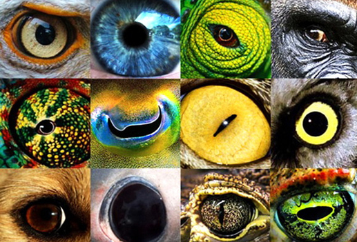
Can you recognize all the eyes in this photo?
Is it just me or is it pretty unrealistic that the species always knows where the food is. In fact, it’s one of the reasons that every species has been doing so well despite how poor their traits and starting conditions are. Now, we’ll finally take away their omniscience and watch their numbers plummet as they have to deal with limited perception like the rest of us.
Perception is a very important limiting factor of species survival. You can only eat the food you find, you can only chase the prey you detect, you can only escape a predator that you notice. There are so many different ways of sensing your environment, and for each method there are so many factors that improve one’s perception, or reduce it (i.e. camouflage). The environment can also impact perception and camouflage, with silty rivers or dark ocean floors making vision a lot less viable than it is for surface ocean dwellers, land dwellers, or particularly aerial organisms.
In fact, we almost cannot continue further in the design of the algorithm until we implement perception. Right now, organisms are just too powerful in their ability to detect food. Anytime I even slightly buff Modelus Specius, he becomes such an effective predator that he eats all of Propagatus Maxima, driving the latter to extinction. This leaves Modelus without any food, so then he goes extinct too. The solution to this is to implement perception, so that Modelus cannot always see where all of Propagatus are at all times.
In this part, we will be removing the following assumption from our model:
- Modelus Specius is a flat, tiny, simple, jelly-like organism that lives at the bottom of the ocean.
- Members of the species will always win combats against smaller individuals, and lose to larger ones (Combat)
- Members of the species always consume 100% of the energy of defeated prey (Metabolism)
- Members of the species can instantly perceive food regardless of distance (Perception)
- Members can reproduce as many times as they want, instantly, with no pregnancy/gestation period. (Reproduction)
- The species reproduces via asexual reproduction, spawning fully developed offspring that can themselves immediately begin reproducing. (Mating)
- The species does not change in physiology as they age (Aging/Ontogeny)
- The species is fully aquatic (Terrestriality)
- Members of the species are solitary and do not cooperate with other species members in any way. (Cooperation/Sociality)
- The species has no parental instincts, and will immediately abandon offspring (Parenting)
- The species is perfectly adapted to its environment and suffers no death or disease from environmental conditions (Environment)
How do Organisms Use Their Senses?
Senses and the sensory system serve organisms in many different ways. Some of the examples of using sensation/perception are:
- Hunting : Using senses to find prey.
- Intimidation : Using senses to intimidate rivals to avoid combat, or determine whether a rival is worth engaging in combat.
- Examining food : Using senses to determine whether found food is good to eat, as opposed to catching food from live prey.
- Communication :
- Using senses for cooperating for hunting/defence/tasks
- Using senses for warning/distress calls
- Using senses for mating rituals
Of these uses, we will only implement the first function for now. Intimidation will be implemented once we’ve added Combat to the algorithm. Examining food will be implemented once we’ve added Scavenging. Communication will be added once we add behaviour and sociality.
Modelling Perception
But how do we actually mathematically represent perception? Well, if you consider perception, it really boils down to two factors: Things that improve an observer’s ability to see a target, and things that reduce an observer’s ability to see a target. We will call these two values Perception and Camouflage.
- Perception represents the ability to sense targets using a particular sense. It represents the strength of the organs involved in sensation.
- Camouflage represents an organism’s “resistance” to being sensed using a particular sense.
These can be influenced by traits of the observer and target organisms, and from traits of the patch/environment (like the murky water example above). Every organism has Perception and Camouflage stats for each sense . For example, the stats of a certain creature for vision could look like:
Vision Perception: 1
+1 from Simple Occuli Eyes
Vision Camouflage: 3
+2 from Cryptic Camouflage Colouration
+1 from Silty Water
Perception vs Camouflage
How do the mathematics of these two stats work? We’ll use a simple ratio of Perception to Camouflage. For example if the species has a Visual Perception of 5, but the target has a Visual Camouflage of 3, then the predator will see the target 5/(5+3) (or 5/8) of the time. This is using a similar concept of ratios of values as we did with speed when determining races to catch prey between predators.
Note that camouflage refers to more than just an organism that has colouration that matches it’s environment. That is an EXAMPLE of camouflage, but here camouflage refers to ALL FACTORS that can make it more difficult for an observer to sense a target.
Perception Range
Another critical limitation of perception is range. There is only so far that you can actually detect organisms at. This means that organisms will now not be able to immediately and consistently detect all prey in the entire patch at all times. Instead they’ll only have a certain range that they can detect prey in. This will greatly reduce the efficacy of predators.
In real life, senses typically are strong when close up but get weaker the farther they are used. This will be too much effort for the algorithm and we’ll just treat the strength of the sense as the same for its entire range, assuming it’s its average strength over that distance.
Sensory Zones
Using these three new traits of Sensory Perception, Sensory Camouflage, and Sensory Range, we will create a model for how senses will work. I call this system, “Sensory Zones”.
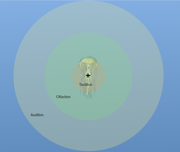
Every organism has a multitude of senses that it uses to experience its environment, and each of these has a range that it can be used at. To mathematically model how these senses detect prey, we will approximate each sense as being like a sphere that extends out from the organism with the organism at its center. Let’s say we have an example organism with senses Tactition, Olfaction, and Audition, with ranges of 1m, 3m, and 5m respectively. What would that look like in zones?
An organism can have multiple spheres, and when they do then they will overlap towards the inside, near the organism. Each of these “regions” of overlapping spheres is referred to as a Sensory Zone.
An important thing to note is that this model ONLY works when senses are approximated using spheres. Cones of vision or different shapes CANNOT work. Instead, the best way to represent a cone of vision is to originally treat it as a sphere, and then reduce the number of targets found in that sphere by a value proportional to how small the cone is relative to that sphere. For example, a cone of length X might have 5% of the volume of a sphere with radius X, which means that to calculate the targets detected using that cone of vision you calculate using the volume of the sphere and then you reduce it by 95%.
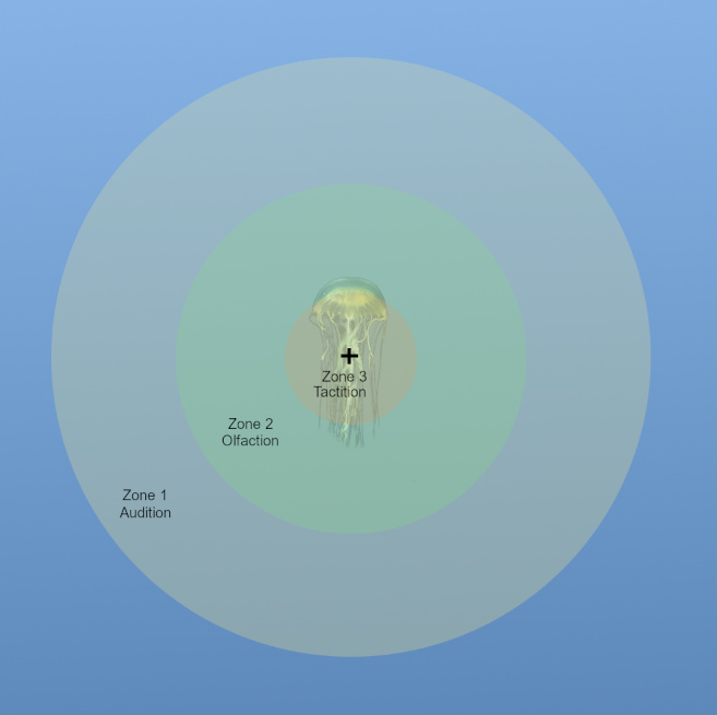
Here we can see how the zones are delineated.
Note that the innermost zone, Zone 3, represents the area where the organism can use either Tactition or Olfaction or Audition to detect prey. As you move out to Zone 2, you lose the ability to use Tactition due to its limited range, and as you move out to Zone 1 you can only use Audition to detect targets in that area.
Each zone has a detection chance. This represents the chance that the observer will notice a target in that zone. This is calculated by taking 1 minus the probability that a target will not be detected by ANY of the senses operating in that zone.
Let’s say we are looking at a prey that is 2m away, meaning he is in Zone 2, meaning only Olfaction and Audition can be used to detect him. The probability that a target will not be detected by any senses operating in Zone 2 is equal to:

Recall that PD is short for predator and PY is short for Prey. Camo is camouflage.
Let’s use some example numbers. Let’s say the predator has a perception of 1 and the prey a camouflage of 1, and the patch has no environmental camouflage. Then the math would come out to:
(1 / (1+1)) * (1 / (1+1)) = 1/2 * 1/2 = 50% * 50% = 25%
Which means that there would be a 25% chance that a given prey would not be detected by either sense in that zone. Thus the “Detection” strength of that zone is 100% - 25%, or 75%.
Updating the Algorithm
How does this tie into the overall algorithm? Well once the algorithm determines the available amount of prey, but before it determines how many the predator can catch uninterrupted (aka without interspecific competition), it must first calculate how many prey the species actually detects.
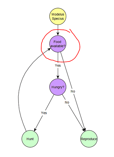
The species will only hunt the organisms it detects, and if it does not detect any more then it will spend the rest of its time reproducing. This means that there could be available prey STILL roaming around the patch, but if the predator never detected them he doesn’t care and goes straight to reproducing. Recall the current behaviour tree of all our species:
The major change here is that, when the species asks itself if any food is still available, it only considers food that is has detected. If he’s hungry but hasn’t any more food, he will think none is available and move to reproducing.
Surveying vs Detecting Prey
So after the algorithm determines the available prey for the species, it calculates how many of them are actually detected. To do this, we first calculate how many prey are surveyed (Surveyed Hunts). This refers to prey that enter one of the sensory zones of the organism at some point, but not necessarily that are detected. To calculate this, we turn to chemistry to borrow the Collision Theory equations (thanks to @tjwhale for the idea).
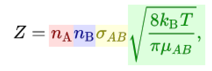
In chemistry this is used to determine how often particles in a confined space bump into each other, and here we’ll repurpose it to calculate how often prey “bump” into the sensory zones of the species. Z represents the collisions per m^3 per second. The term in red represents the population density of the predator, and the term in blue the population density of the prey. The yellow term represents the reaction cross section, which is equal to:
pi * (Predator's sensory zone radius + Prey's body radius) ^ 2
This takes into account how big the predator’s sensory zone is and how big (or small) the prey is. Finally, the green term can be simplified to just be the average speed of the predator and prey. For now, we’ll assume that while surveying, the predator and prey both move at half their top speeds. Rewriting this in our terminology gives us:
![]()
But recall this is just prey surveyed per m^3 per second, so we need to multiply it by the volume of the patch and the number of seconds in a month to get the total number of prey surveyed.
Finally, when you have the total number of prey surveyed by each of an organism’s sensory zones every month, you then multiply that by the detection strength of that zone to see how many of those surveyed prey are actually detected by the predator. This finally yields the Detected Hunts, which the species then uses to determine how much to hunt. After this comes the calculation of Uninterrupted Hunts, Caught Hunts, and all the rest that I’ve already explained.
Major Bugfixing and Overhauls
However, before we get to the demo, this would not be a complete part before I rant about the recent bugfixes and code overhauls I did! It seems like the changes I made in Part 7 and now Part 8 were pretty damn major, and I’ve been finding bug after bug since then. I’ve solved as many of them as I’ve found, including some pretty major ones. One of the ones I caught was a bug where species were only attempting as many hunts that they required assuming all of them would be caught, and not taking into account the possibility for failure rates. This was a pretty big bug and came from my misunderstanding of the hunting breakdown. Now the species attempts as many hunts as it needs until it gets the number of successful ones that it requires (unless constrained by time or available prey). So if a species needs 500 hunts and has a failure rate of 50% when hunting, he will spend time attempting 1000 hunts to get the 500 successes he needs.
Demo
With the new features in and the bugs ironed out, let’s see how the simulation turns out!
Modelus Specius will have tactition and olfaction as his senses. Tactition will be a stronger sense (+2 Perception, 5cm range) but olfaction will have a farther range (+1 Perception, 25cm range). His intraspecific competition rate was also increased 5x to help curb his effectiveness as a predator.
All species will have a bit of natural camouflage (+1) towards being sensed by tactition and olfaction. The camouflage to tactition could be the fact that these creatures are all very soft-bodied and thus harder to perceive touching. The camouflage to olfaction could be that they are very small and simple and do not excrete too many chemicals or pheromones into the environment. The environment also has some camouflage to these two senses (+1), representing water currents blowing away scent trails and perhaps getting in the way of touch reception.
There are of course many other senses I could’ve included, like audition and gustation and vision, but I’ll hold off on those for now to keep the model simple.
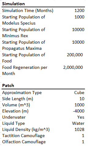
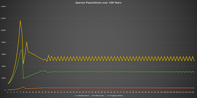
This time I ran the simulation over 100 years (note the unit is months on the bottom axis). I also increased the starting populations by a lot. All species also had their energy yield (when consumed) reduced from 100 calories to 10 calories, meaning Modelus needs to hunt 10x as much as a carnivore. Note that this is a typo on the screenshots below which still show 100 calories as the energy yield.
The final population values are:
- Minimus Rex: 56,264
- Propagatus Maxima: 31,141
- Modelus Specius: 3,597
When running the simulation, we can see we reach an equilibrium after 2 years. Perception does definitely drag out the time it takes for major events to occur, like the food supplies running out or predators overhunting prey, but we still do see the same patterns.
The initial spike is the initial growth of the “herbivores” (Propagatus and Minimus) before the food shortage kicks in. It’s interesting to note that the big famine causes the carnivore, Modelus, to also take a hit to its population. Another interesting thing is that immediately after the big famine, Minimus Rex’s population spikes up again, but then hits a second famine and crashes back down again. I’m guessing this is because immediately after the famine Minimus is still much higher in population than Propagatus and thus has a competitive advantage in catching the glucose clouds, but as Propagatus’ population grows Minimus loses this edge.
Eventually, after 2 years, equilibrium kicks in and we can see that all three populations stabilize. We can start to see the typical predator-prey cycles taught in ecology at this point, with prey and predator populations fluctuating in response to each other. Minimus Rex is also affected by this, since he competes with Propagatus for food. It will be interesting to see how these predator-prey dynamics change once we create a more complex food-chain, with predators feeding on predators.
Although it may not look very different, this part greatly helped to curb the effectiveness of predators in the predator-prey cycle. It’s now much more difficult for a predator to completely eat all of its prey in the patch, since he would need to actually detect all of them. This part also greatly increases the ability for evolution to impact the results of hunting. Now all of the traits of perception, camouflage, and range for every sense can play a huge role in how many prey are detected by each predator in the ecosystem!
That’s all for this part! It took a lot of coding and bugfixing but it’s finally done. Stay tuned for the next post. Chances are I will dive more into perception and sensation with a sub-part if I find that there was something I missed, or I might do a special version of a Simulation Demos sub-part. Once those sub-parts are done, we’ll then move on to the next big topic!
Summary
New Performance Stats
Surveyed Hunts
Detected Hunts
New Traits
Perception, Camouflage, and Range for the following senses:
- Tactition, Gustation, Olfaction, Audition, Vision, Magnetoreception, Thermoreception, Electroreception
Topics for Discussion
- All comments and feedback are welcome!
