Episode 1 – Population Algorithm
“How does one calculate the effect of an evolution on a species?”
Part 1: Population
Before we do anything else, the very first thing we must determine is how to calculate the effect of any change, mutation, or evolution on a species. Once we figure that out, we can proceed to Episode 2, where we calculate several different evolutions for a species, and then choose the best one.
To address this first question, the answer lies in population. Population is the ultimate success metric for life, since population growth is life’s ultimate goal. Evolution by natural selection is rooted in the principle that the guiding force of life is to propagate your DNA, and the medium of DNA is population. Have more offspring, and you have more copies of your DNA. Ensure that your offspring have more offspring, and you have further copies of your DNA still. Even the acquisition of food is only a means to the end of sustaining and multiplying your population. Population growth and decline is also what determines the appearance and disappearance (extinction) of species. As such, we can see that population is the central metric to track for a species to measure its performance, a convention already in wide use in modern science.
So, within one paragraph we already know the conclusion of this episode: You calculate the effect of an evolution on a species by seeing how it changes its population in future generations. In Episode 2, we will look at how you can assign several different evolutions to a species, calculate which one produces the greatest growth in population, and choose that one as the mutation chosen by Auto-Evo.
However, it’s not as easy as just saying “by seeing how it changes its population in future generations”. How exactly does that work? There is a lot of work still left before we can move to the next episode, since the rest of this episode is all about figuring out how exactly any given evolution will change the population. We will need to figure out exactly what stats of the creature will cause exactly what changes to their population and by which exact mathematical relationships. This might seem difficult at first but remember, we have several strategies described earlier to help make this process easier.
Mathematical Aside
Discrete vs Continuous Modelling?
Before we can begin creating the algorithm, we must answer a fundamental mathematical question: Do we make a discrete or continuous model?
Discrete Model
A discrete model assumes that changes only take place at specific intervals. For example, a discrete model for population growth would take the current population, and an annual growth rate, and tell you what the population would be after 1 year:
Population at Next Year = Growth Rate * Population at Current Year
For example: 110 = 1.1 * 100
We can also rewrite this equation using function notation:
n[t+1] = R * n[t]
Where:
t is the current year
t+1 is the next year
n is the population
n[t] is population at the current year
n[t+1] is the population at the next year
R is the growth rate
If R is 1.1, that is equivalent to 110%, or that the population is growing by 10% every year. An R of 0.9 is equal to 90% and means that the population is shrinking by 10% every year. An R of 1.0 means a growth rate of 100% which means that the population is staying exactly the same (such as if exactly as many organisms died as were born).
Benefits
The benefit of discrete models is that they are simple and easy to understand and do the math for, as they are the usual way we do simple math at the high school level or in everyday situations. It also makes it pretty easy to track information at each timestep to monitor changes in the environment.
Drawbacks
One consequence of this discrete method though is that it assumes that none of the births in that year birthed any of their own. Its equivalent to saying that all the births happened exactly at the last moment of the year, or all right at the beginning and then no other births for the rest of the year.
Why is calculating at specific intervals an issue? It’s because this leads to problems no matter how large or small we make the time interval. If we make the interval too large such as 1 year, this could lead to less realistic outcomes. Perhaps the species has very short lives and within a year they could have offspring and then those offspring could have their own offspring. However, a 1 year interval wouldn’t allow for that, since the offspring would have to wait a minimum of 1 year before the calculation could run again. If we make the interval too small, such as 1 week, this could lead to very computer intensive calculations that would slow down the game. The game would have to run the entire Auto-Evo calculation 52 times just to simulate growth over a single year, and that’s only for one species!
Continuous Model
The alternative to this are continuous models. This is where you calculate a continuous rate of change over the interval, meaning that offspring born within a year could have their own offspring. For example, a continuous model for population growth will give us the change in the population at any given instantaneous moment:
Rate of Change of Population at Current Moment = Growth Rate * Population at Current Moment
Or with proper function notation:
dn[t] / dt = R * n[t]
Where:
dn[t] / dt is the change in population at a given instant
R is the growth rate
n[t] is the population at a given instant
You then would calculate this multiple times to find the overall change of a population over 1 year, and it would give you a slightly different answer than a discrete model, but still pretty close. The difference could even be larger based on the parameters.
Drawbacks
What are the downsides of continuous modelling? Well, how do you use equation that gives population change at any given instant to calculate the total change over an entire year? Surprise surprise, to anyone who hasn’t done this in college, its calculus. It means our model would have to involve a lot of calculus, and that would make things a LOT more challenging (especially for me since it’s been a few years since I’ve studied calculus).
Which is the Better Model?
So the question is, do we use a discrete model, or a continuous one?
My vote is for a discrete model. It’ll save us the headaches of constantly having to work with calculus, and we can hopefully try to strike a balance with the time intervals where it’s not too long and not too short to produce any of the problems listed above. It also allows us to easily track information between time intervals and display these to the player.
The interval that I think would be the best balance is 1 month per interval. Most species on Earth have lifespans that are at least 1 month long. In fact, almost every exception to this rule is in microbial organisms. Perhaps we can make two different algorithms, with one that uses 1 month timesteps and one that uses smaller timesteps? The smaller timestep model would only be used for microbial life, which wouldn’t create any overlap since all microbial life stops being simulated during the 2D-3D transition of the Multicellular Stage.
Initial Algorithm
Assuming we create a discrete model, we can finally get started on the algorithm.
Let’s create a list of all the assumptions we are making to create our extremely simple and easy to understand scenario.
Current Assumptions
- Modelus Specius is a flat, tiny, simple, jelly-like organism that lives at the bottom of the ocean.
- The species is always fully satiated with food and water (Nutrition)
- The species is equally distributed/dispersed across the world (Demographics)
- The planet is one giant ocean of equal pressure water that is equally accessible to the player (Geography/Terrain)
- Members can reproduce as many times as they want, instantly, with no pregnancy/gestation period. (Reproduction)
- The species reproduces via asexual reproduction, spawning fully developed offspring that can themselves immediately begin reproducing. (Mating)
- The species does not change in physiology as they age (Aging/Ontogeny)
- The species is fully aquatic (Terrestriality)
- Members of the species are solitary and do not cooperate with other species members in any way. (Cooperation/Sociality)
- The species has no parental instincts, and will immediately abandon offspring (Parenting)
- The species is perfectly adapted to its environment and suffers no death or disease from environmental conditions (Environment)
In future parts, we will always have a list of all current assumptions at the BEGINNING of the post, and we will explain what assumptions are being “peeled away” (replaced with realistic mechanics) in that part. This will hopefully ensure we understand the algorithm every step of the way.
Using our simple model, here’s a simple place to start. The following equation calculates the change in population over one timestep (1 month):
Population = Initial Population + Births - Deaths
OR
P = Pi + B – D
Okay, easy enough. Now let’s break down how to calculate Births (B) and Deaths (D).
Births
What determines how many births there are in a timestep?
First we look at how many individuals CAN reproduce (Available Reproducers). For example, in the human population this would be around 50%, since only females can reproduce. However, in Modelus Specius, there are no sexes and all members are capable of asexual reproduction, thus making the available reproducers 100% or 1.0.
Then, of those that can reproduce, how frequently do they actually reproduce (Mating Frequency)? In some species, this is influenced by factors such as sexual competition. However, in our simple Modelus Specius, this is only limited by how often they can reproduce within physical limits. In fact Modelus Specius spends 100% of its time just reproducing. The only thing that limits it is how fast the cells can replicate to reach double their original number and spawn an offspring. This means Modelus Specius uses Budding to reproduce. Let’s say that the cells in Modelus Specius replicate fast enough to allow it to reproduce once per month.
Then, when these members reproduce, we need to know how many offspring are produced (Litter Size). Since Modelus Specius reproduces by Budding, we’ll say it only produces 1 offspring.
Thus we can break Births down into:
Births = Initial Population * Available Reproducers * Mating Frequency * Litter Size
And with our example numbers
Deaths
At this point, our model is so simple that members of Modelus Specius only die from old age. Yes, I know, what does it mean to die of old age? For now, we’ll keep this old age model extremely simple and simply say it’s natural diseases that occur and kill organisms after a certain amount of time. In a later part we’ll revisit it and replace it with a realistic model of ontogeny and aging.
Let’s say that Modelus Specius has an average lifespan of 3 months. Some die at 2 months, some live to 5 months, but on average they live 3. We can then assume that with a starting population of 100 newborns, 100% of them will die in 3 months, and 33% of them will have died by the first month. At the moment we will not be keeping track of multiple generations. Also, in real life it’s more common for deaths from old age to increase in likelihood when you get older, but we are also ignoring that for the moment. From this we get:
Deaths = Initial Population * 1 / Lifespan
Updating the Equation
Now plugging these back into our equation, we get:
Births = Initial Population * Available Reproducers * Mating Frequency * Litter Size
Deaths = Initial Population * 1 / Lifespan
Population = Initial Population + Births - Deaths
Visualizing the Algorithm
As we progress through the series, we NEED to keep track of our algorithm as we build it up. This is so that we always are able to understand it as we’re building it and we never start to get confused by how complicated it is. To help with this, I think it’s better to visualize it in several different methods. We will use these methods throughout the series as we build the algorithm.
Equations
The first method of representing the algorithm is simply to write out the list of equations we are using. This is what we have so far:
Births = Initial Population * Available Reproducers * Mating Frequency * Litter Size
Deaths = Initial Population * 1 / Lifespan
Population = Initial Population + Births - Deaths
Another way of looking at the algorithm is to draw a visual diagram of what is happening with the species under Auto-Evo. The two diagrams we’ll use are the Life Cycle Diagram, and the Flow Diagram.
Life Cycle Diagram
The Life Cycle Diagram shows the order of events in the lifespan of an organism of the species. Here is the typical Life Cycle Diagram used in biology:
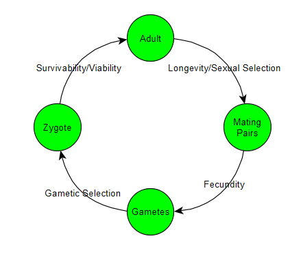
Notice how from one generation to the next, there are actually several steps at which members can die and natural selection can do its work. Not all of natural selection is involved in whether you survive to adulthood, which is the part people usually think of. There is also the “competition” of which adults get to reproduce (especially if they need to find mates, which is sexual selection), how fertile and successful those reproducing adults are, and how successful the gametes are in fertilizing. However, most of these are irrelevant in our current simple model.
A cool benefit of this diagram is that it also can show us what order calculations are done by the algorithm. Let’s rewrite the diagram to show our current algorithm.
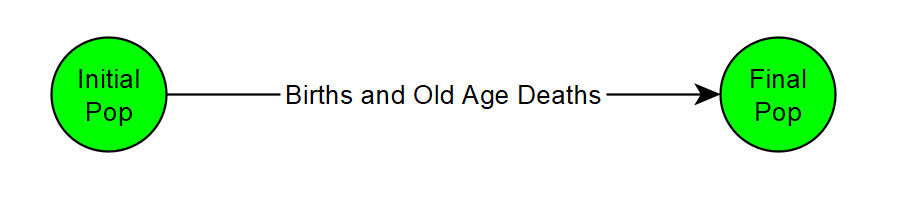
We start with the initial population of the generation. Some of them birth new offspring, and some of them die of old age. Some can birth an offspring and then die of old age. Once we factor in the births and deaths we get the population of the next timestep.
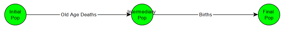
However, there is one problem with this. The order of calculation is very important. What if you die of old age before you reproduce? The current model does not allow for that. This might seem trivial now, but it will become very important in the future when an individual might die of starvation before they can give birth, which is an important factor of natural selection. Let’s re-order our equations to first kill off all the members who are dying of old age, and THEN have the survivors reproduce.
Deaths = Initial Population * 1 / Lifespan
Intermediary Population = Initial Population - Deaths
Births = Intermediary Population * Available Reproducers * Mating Frequency * Litter Size
Population = Intermediary Population + Births
What does this now look like?
Flow Diagram
Another way to visualize the data is with a flow diagram. This simply shows all the different factors that increase (inflows) and decrease (outflows) the population every timestep. It can even be expanded to show what variables affect each of these flows. Here’s a simple mockup:
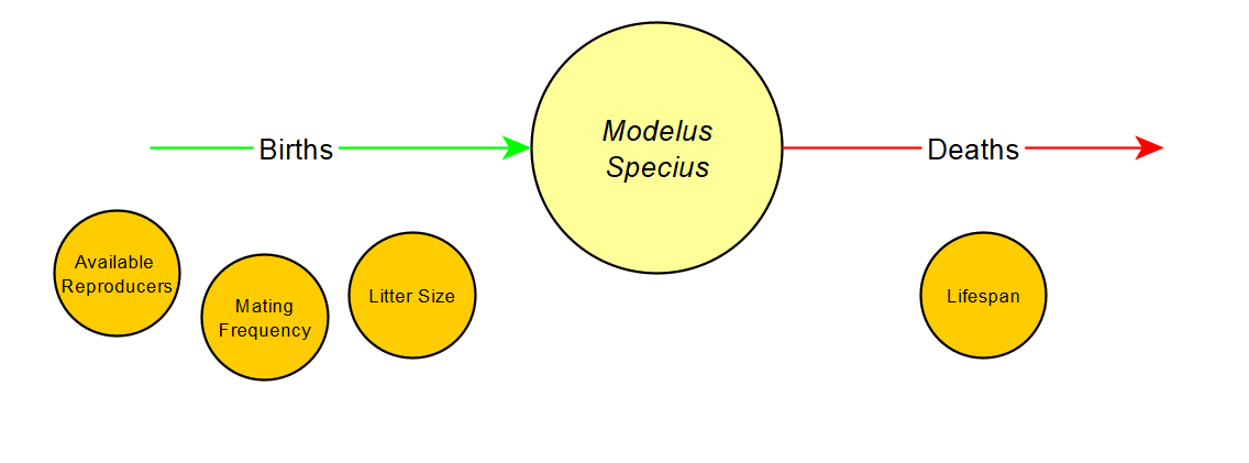
I have a feeling this one will not be as helpful once the model starts getting more complex, but I’ll keep it around for now.
Demo
I think Excel is good for visualizing the data, but ultimately a scripting language like Python is needed to make a demo of the algorithm (some functions are just not possible or too complicated in excel). Using Python, I made a script to model the algorithm we have so far. At the end it spits out a monthly report of the environment as a CSV file.
Starting Conditions
- Simulation Time = 24 months
-
Modelus Specius
- Starting Population = 100
- Available Reproducers = 1.0
- Mating Frequency = 1/month
- Litter Size = 1
- Lifespan = 3 months
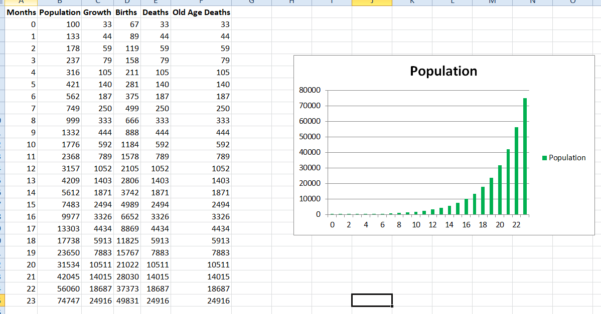
Notice that the population grows exponentially, since there is nothing to limit it. In future parts we will fix this by introducing more elements of the natural environment to produce a more realistic outcome.
Summary
Every part will end with the Summary. The summary will have two lists and a compilation of all the unanswered questions that need to be addressed for that part. This is to keep a running tally of all new stats we add to the algorithm and what design decisions need to be discussed next. The first will be a list of any new Performance Statistics introduced in that part. These are stats that help the player track the success of their species, such as population, births, deaths, starvation rate, etc. Performance statistics change from month to month. The second is a list of Traits introduced in that part. These are stats of the species that are defined in the OE. Traits can only change through evolution, and are constant from month to month. The first post will have an appendix to keep a record of all Performance Statistics and Traits as they are added.
Performance Statistics
Population
Births
Deaths
Old Age Deaths
Traits
Available Reproducers
Mating Frequency
Litter Size
Lifespan
Topics for Discussion
- Do we go with a Discrete or Continuous Model?
Finally, I’d just like to take a minute to point out how incredibly useful I think it is that we are starting with such a simplified model. Even with such a simplified starting model, look how complicated things have already gotten! We’ve discussed discrete versus continuous mathematical models, calculus, different types of natural selection, different types of mathematical modelling of population growth, different visual representations of the auto-evo process, and introduced various variables to construct our initial equation, and this is only the first part of the first episode! Clearly we will have to take things slowly and make sure everything makes sense and fits together along the way.